ATSC 113 Weather for Sailing, Flying & Snow Sports
Determining the temperature at your mountain elevation
Learning goal 6h: Determine the temperature at your elevation by interpolating from pressure-level maps
Temperature forecasting in the mountains is best divided into a two-step process. First, vertically adjust (interpolate) the temperature from a low-level pressure map (e.g. 85.0 kPa) to the elevation you are concerned with, giving you the free-air temperature (defined below). Second, make an adjustment to that temperature based on the heating or cooling that may be occuring at the ground surface. We cover the first step in this learning goal. The second step will be covered in Learning Goal 6i.
Vertical interpolation
Suppose you know a quantity such as temperature at each of two locations, but you want the temperature for an in-between location. The process of estimating that quantity at the in-between location is called interpolation.
Pressure levels in the atmosphere can be related to different
mountain elevations (Learning Goal 6n). Pressure-level maps are
generally only produced for certain pressure levels (usually 85.0kPa,
70.0kPa, and 50.0kPa). However, snowsports happen at all elevations on
the mountain! Therefore, it is helpful to interpolate
temperatures in
between the pressure-level maps to get the best temperature forecast
for your altitude.
-
Free-air temperature
The free-air temperature is the temperature at a particular level of the atmosphere, assuming no heating or cooling effects from the surface. We'll discuss how to account for those effects in Learning Goal 6i. This will improve the accuracy of our temperature forecast for our elevation on the mountain.
-
Dry adiabatic conditions
Under dry adiabatic conditions, temperature decreases with height at a rate of about 10°C per 1000 metres (dry adiabatic lapse rate = 9.8°C/km). It's generally appropriate to assume a dry adiabatic lapse rate when the modelled atmosphere is not close to saturation (below 80% relative humidity), and (a) if the winds are moderate or strong (~40 km/h or greater), (b) in the daytime during the spring, or (c) in some cases during the afternoon on sunny winter days. If the humidity is exactly 80%, then look at surrounding areas to see if humidities are generally drier than 80%.
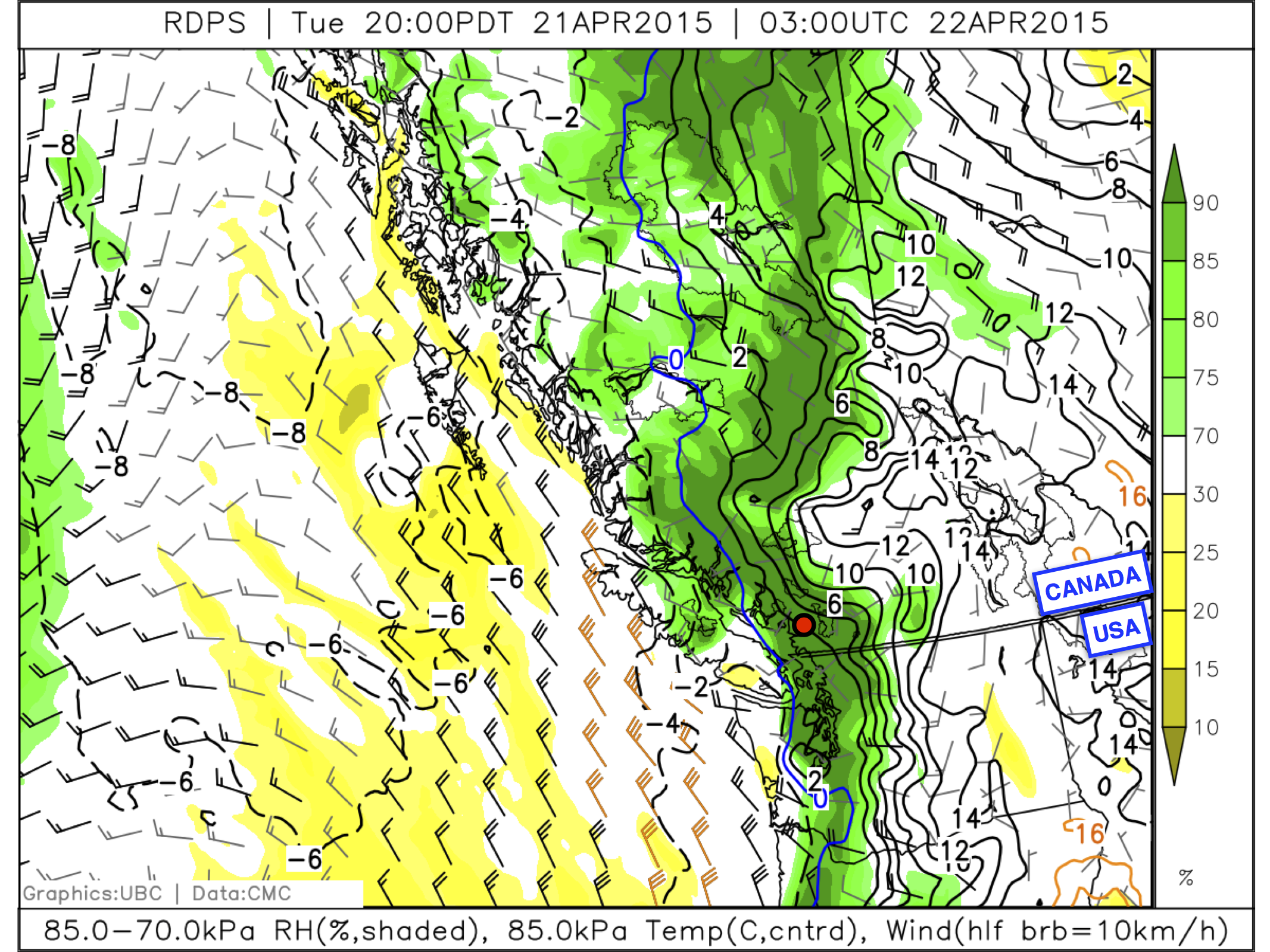
Fig. 6h.1 An 85.0-kPa pressure-level map showing temperatures (contoured), relative humidity (yellow and green shading according to scale), and wind barbs. Grouse Mountain is marked with a red-in-black circle, just to the north of Vancouver. (Credit: West)
Scenario: you want to go skiing at Grouse Mountain (elevation ~1000 m) in the North Shore Mountains, and you have access to an 85.0-kPa (approximately 1500 m, but use interpolation tool below for exact number) pressure-level map to forecast temperature (like the one in Fig. 6h.1 that shows temperature, relative humidity, and winds). Grouse Mountain is indicated with a red-in-black circle. If you follow the black contour line (isotherm) that passes through this circle northwards, you will see that it represents a forecasted temperature of 2°C.
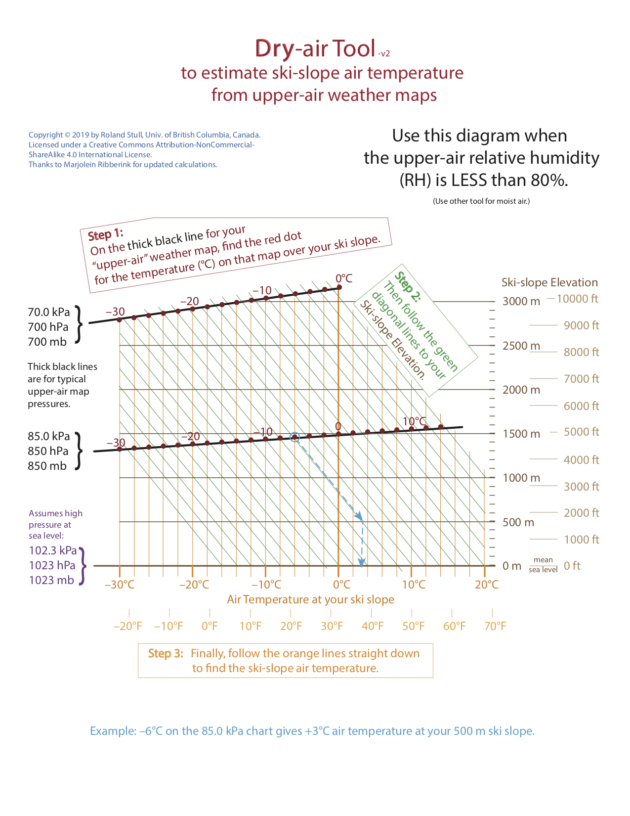
Fig. 6h.2. A tool to allow easy estimation of temperature at your ski slope, for relatively dry conditions. (Credit: Stull)
We need to interpolate from this "known" temperature at a height where the pressure is 85.0 kPa down to a height of 1000 m for the ski slope. The easiest way to do this is to use the graphical tool for dry air (Fig 6h.2), which does not require you to do any calculations. [CAUTION, the light-blue Example in that figure is for a different case than the one we are using here.]
Method:
(1) On the dark black line for 85.0 kPa, find the dark red dot for +2°C.
(2) From that red dot, follow (or go parallel to) the green diagonal lines down until the elevation of 1000 m.
(3) From that point, follow the orange lines straight down to read-off the air temperature. The answer is approximatly 7°C at 1000 m elevation on Grouse (warm day!). This is a good starting point for a temperature forecast. -
Wet adiabatic conditions
When the atmosphere is saturated (100% relative humidity), temperature decreases more slowly with height. Under wet adiabatic conditons, temperature decreases at a rate of approximately 6°C per 1000 m (6°C/km) in mild air, but the rate of decrease varies with temperature. In the model-simulated atmosphere, you can make this assumption when forecasted relative humidity is greater than 80%. If the humidity is exactly 80%, then look at surrounding areas to see if humidities are generally moister than 80%.
Looking again at the 85.0-kPa forecast map (Fig. 6h.1), we see relative humidity is greater than 90% for Grouse Mountain. In this situation, it is more appropriate to use the wet adiabatic lapse rate. Again, you can use a graphical tool to estimate the air temperature without doing any calculation. This time, use Fig. 6h.3 to do the interpolation for moist air.
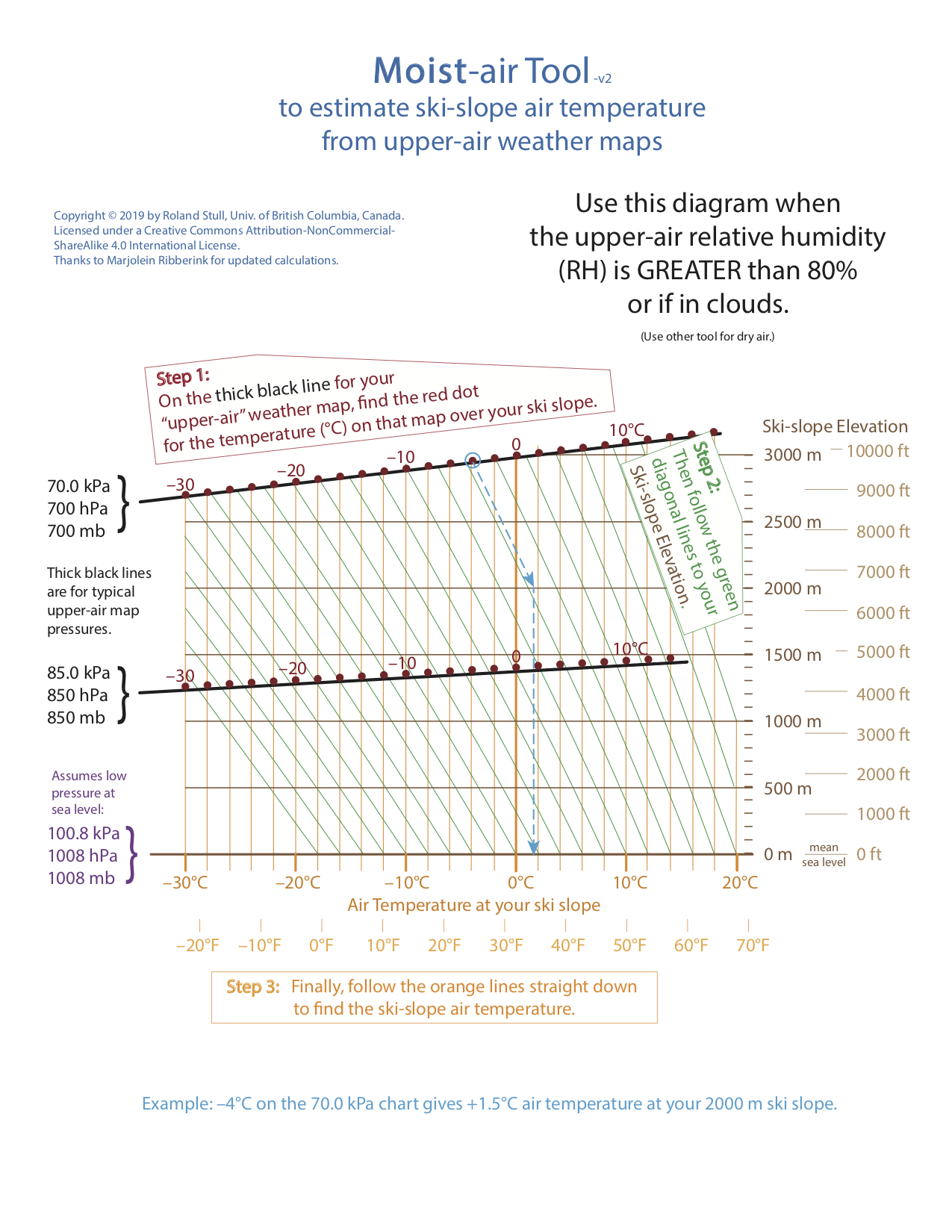
Fig. 6h.3. A tool to allow easy estimation of temperature at your ski slope, for humid and foggy/cloudy conditions. (Credit: Stull)
[CAUTION, the light-blue Example in that figure is for a different case than the one we are using here.]
Method:
(1) On the dark black line for 85.0 kPa, find the dark red dot for +2°C.
(2) From that red dot, follow (or go parallel to) the green diagonal lines down until the elevation of 1000 m.
(3) From that point, follow the orange lines straight down to read-off the air temperature. The answer is approximatly 4.5°C at 1000 m elevation on Grouse. This is a good starting point for a temperature forecast.
Note: If quiz or exam questions require temperature interpolation, we will provide these two graphs.
-
Stable conditions
In some situations, we may have a lapse rate that is more stable than the wet adiabatic lapse rate. In other words, the temperature decreases very slowly with height, or, in some cases, increases with height (an inversion, Learning Goal 6c).
Inversions typically occur locally within valleys in the overnight and morning period in the winter, and during Arctic air outbreaks (Learning Goal 6l). There's no specific lapse rate assumption you can make in these cases, as inversion lapse rates vary widely. Just keep in mind that temperature can increase rapidly as you go up the mountain, and conversely, it can decrease rapidly if you are heading downhill to lower elevations.
At mid to upper elevations, a very stable temperature profile is common during a frontal passage, even if there is moderate to heavy precipitation occurring with the front. The temperature is usually nearly constant with height. Thus, during a frontal passage, no vertical interpolation is needed, and the temperature at your elevation should be very similar to that of a nearby pressure level.
Keywords: free-air temperature,
interpolation
Figure Credits: Howard: Rosie Howard, West: Greg West, Stull: Roland Stull