Lab #9 - Basics of Electromagnetic Induction
Frequency-domain EM

TA: Gudni Rosenkjaer

Overview:

Elementary circuits can be used to simulate the responses for EM surveys. In this lab you are provided with a MATLAB code that allows you to explore the character of the responses under different conditions. The basic principles for EM induction have been provided in the notes and you will use those notes to accompany the abbreviated text provided here. In this lab you will use a MATLAB code to better understand the the fundamentals of EM induction.

Background for EM induction & the EM-31:

One of the simplest electromagnetic devices is the EM-31 system. Read the overview of the system, here.

The EM-31 consists of a transmitter (Tx) and a receiver (Rx) which are mounted at the ends of a 3.6m long boom.

Transmittor
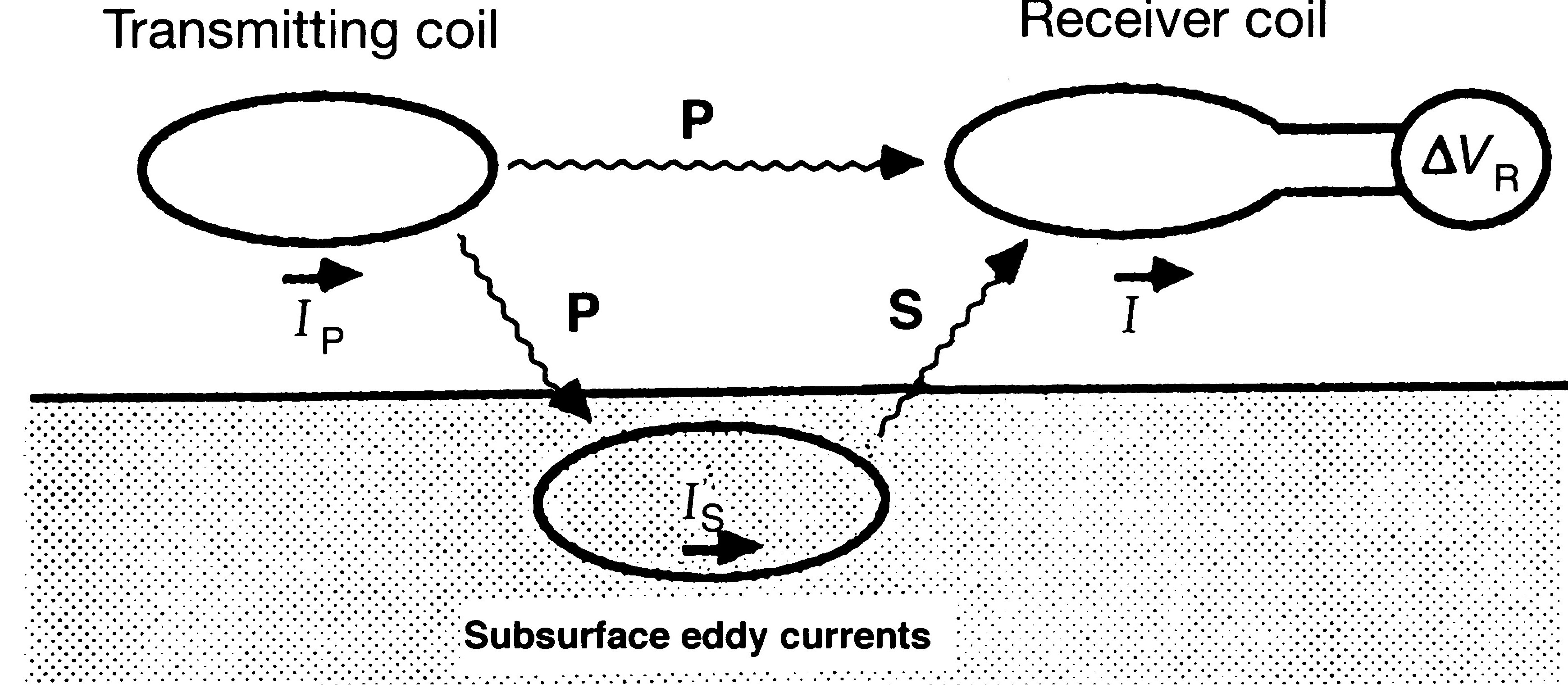
- Carries a sinusoidal (or harmonic) current of frequency f=9700 Hz. This sets up a time varying magnetic field everywhere in space. This is called the primary field Hp. A circular loop of current generates a magnetic field that is the same as that due to a magnetic dipole, with a dipole moment m=IA where I is the current in the Tx and A is the area of the Tx. The representative dipole is located in the center of the loop and is orientated so that it is perpendicular to the plane of the loop. The strength of the magnetic field is that of a magnetic dipole with moment m, and hence it falls off as 1/r^3.
Receiver
- This is also a loop of wire. There is an EMF (Voltage) induced in the receiver that this related to the time rate of change in magnetic flux.

If the EM31 were operating in a vacuum then the magnetic field at the receiver would be Hp, the primary magnetic field. For the EM31 the Tx and Rx coils are co-planar (in the same plane). The Rx is sensitive only to magnetic fields that cross its plane, so the co-planar geometry is one of maximum “coupling”. If the Rx coil was rotated 90 degrees so that it was perpendicular, then no magnetic field lines would cross its plan and no voltage would be induced.

Conductive body in the earth
- We can represent a conductive body by a loop of wire that has a resistance (R) and a self-inductance (L). The time-varying magnetic field due to the Tx impinges upon the loop in the earth and sets up an EMF in it. This causes an electric current to flow in the loop. The orientation of the loop with respect to the incident magnetic field (Hp) will determine how much EMF is induced and hence the amount of current. The current flowing in the loop will produce a dipole magnetic field (just like what happened with Tx). The magnetic field produced by this underground conductor is called the secondary magnetic field, Hs. The secondary magnetic field can be detected by the Rx.

The data
- The data recorded by the receiver are the ratio of the Hs/Hp. For frequency domain systems this is a complex number which can be written as a combination of:
  - Real (or In-Phase)
  - Imaginary, (or Out-of-Phase, Quadrature)
- Each datum is plotted at the mid-point between the Tx and Rx.
- The strength of the signal depends upon :
  - Conductivity and inductance of the target. Here you use R (resistance) and L (inductance) to characterize the target.

fem3loop.m

In this lab you will be using the MATLAB program fem3loop.m to simulate the inductive response of simple burried tagets. The MATLAB code can be downloaded here.

Users have the ability to input the following parameters though an input file (fem.txt). An example of the file is given below:

0.1 2000 !! inductance and resistance of the target
0 0 2 !! easting, northing, and depth of the target
0 90 !! inclination and declination of the normal vector of the target
4. 1 10000 !! Tx-Rx loop separation, height above ground, and frequency
-10 10 0.25 !! min, max, and interval of observation grid in easting
-10 10 0.25 !! min, max, and interval of observation grid in northing

A sample input file is provided for you to start with. It can be downloaded here. You can then change the input parameters for different scenarios.

The orientation of the target is controlled by the Inclination and Declination of the normal vector of the target. These have the same definition as in magnetic surveying. A horizontal loop has a normal vector that points in the vertical direction and hence has an inclination of 90 degrees. A vertically oriented loop has a normal vector that points horizontally and hence has an inclination of zero. The declination is the angle from north. A declination of 90 degrees means that the axis of the loop is pointing in the easting direction.

The Tx and Rx are separated by a value you can control. Also you can also control the height at which data are acquired and the frequency of the transmitter. Data are collected over a rectangular grid and you can control the station and line spacing.

To run the code, you must first change the MATLAB directory to the same folder where you saved the fem3loop.m file. Then simply type "fem3loop" into the Command Window. You will then be prompted to select an input file.

The program will produce three plots for each run:

The frequency response of the target. The frequency point corresponding to your input is indicated so that you know which frequency range you are in.
Map plots of the real (in-phase) and imaginary (quadrature) components of the anomalies, respectively.
An east-west profile of the same anomalies in the same plot.

Tasks

Using the fem3loop program, complete the following seven tasks. Answer the questions contained in each task.

Sketch the east-west cross-sectional view of the setup in the above input file. Place the Tx and Rx in their locations for the datum at x=-4m. You will use this type of figure for your plots in the following sections.
Run the program using the sample input file and examine the plots. Concentrate first on Figure 3; the east-west profile.
- Consider the datum at x=-4m. Use your 2d diagram with true location of the Tx, target, and Rx on which to do the following.
  - Sketch the Tx with an increasing current going clockwise when looking from above. Sketch and label the primary magnetic field.
  - Sketch how the fields interact with the target and the direction of the induced currents in the target.
  - Sketch and label the secondary magnetic field.
  - Use the sign convention that the observed datum is positive when the secondary field is in the same direction as the primary field at the receiver. Show that your datum is in agreement with the computed value in Figure 3.
- Repeat the exercise above for the observation points: x=-2, x=0, x=2, x=4. Do your predicted results agree with what is shown in Figure 3?
The above work is geometrical and applies equally well to the Real and Imaginary portions of the recorded data. That is, both Real and Imaginary transect plots will have the same characteristic shapes. Their relative amplitudes however are determined by the conductivity and frequency of the target. More precisely it is the dimensionless quantity wL/R. Evaluate this number for the input file provided. Use the diagram in Figure 1 to evaluate the theoretical ratio of Real/Imaginary amplitudes for this example. Now use Figure 3 to see if your recorded data are in accordance with that number. Repeat this exercise using R=20000 (now we have a poor conductor).
Change the inclination and the declination of the target to be I = 0, and D = 0. Sketch the orientation of the Tx, Rx and the target for the datum at x = 0m. Run fem3loop for this new setup. What is the explaination of the result you see in the E-W profile over the target.
Return to the original settings (I = 0, D = 90). Examine how the data changes with the depth of burial of the target. Investigate z=2, 20 in steps of 2 meter increments. How does the amplitude of the anomaly change as a function of depth? What are the most significant changes in the character of the anomaly? How are the zero crossings of the data along the profile affected?
Again return to the default settings but alter the data acquisition strategy. Slowly increase the station and line spacing. What is the largest station spacing that can capture the anomaly?