EOSC 350

Lab 9 - DC Resistivity

Introduction

In this lab, we work with DC resistivity survey using a synthetic data set created from a 2D synthetic model (blocks in half-space). You are expected to load and understand the data, read the apparent resistivity pseudo-section, and carry out the inversion in attempt to recover the true model.

Download the package containing the files used in this lab from here (Windows executables). Unzip and copy the files in one file folder. You need to launch cmd.exe in Windows and change the directory to this working folder to run the inversion program; other files can be opened or launched by mouse click.

There are 6 files in the package:
dcinv2d.exe : DC 2D inversion program
dcinv2d.inp : inversion parameter file
dcip2d-data-viewer.exe : DC 2D data viewer
dcip2d-model-viewer.exe : DC 2D model viewer
libiomp5md.dll : dynamic-link library required by the inversion program
Mystery_dc_uncert.obs : DC data file

DC Data

Open the DC data file Mystery_dc_uncert.obs in a text editor. Each row corresponds to a DC resistivity reading. The first 4 columns of the data file are for the locations of current and potential electrodes. The fifth column is the DC data. The last column is the error for the data.

Q1: What is the unit of DC data?
A. S/m B. Ampere C. Ωm D. Volt E. msec F. mV/V G. % H. meter

Open dcip2d_data_viewer; click File -> Open; in the pop-up dialogue box, browse Mystery_dc_uncert.obs for dcip2d data file; select DC for data type; click OK to proceed.

Q2: This map shows the DC data as a pseudo-section of apparent resistivity. What is the unit of the color on this map?
A. S/m B. Ampere C. Ωm D. Volt E. msec F. mV/V G. % H. meter

Find the lowest apparent resistivity on the map. Click the circle mark for that datum to activate Data Properties dialogue box. Look at the electrodes on the surface.

Q3: What type of array is used in this survey?

Q4: What are the positions (x-coordinate in meter) of the current electrodes (A & B) and the potential electrodes (M & N)?

Q5: What is the value of that datum and its apparent resistivity?

Q6: Provide a formula that transforms the potential difference measured at M and N electrodes to the apparent resistivity. Find the geometric factor of this particular datum. What parameters can cause the geometric factor change across the pseudo-section?

Q7: Under what condition, the apparent resistivity calculated from the data is equal to the true resistivity of the ground?

Q8: Sketch a cross section with electrodes A, B, M, N for this type of array on the surface. Draw current flow lines and equipotential lines underground (assume a uniform half-space model).

Click other circle marks on the map; the current and potential electrodes will move around.

Q9: In this survey, the locations of the current electrodes are (choose: fixed or variable); the locations of the potential electrodes are (choose: fixed or variable); the spacing between the two potential electrodes is (choose: fixed or variable). When the current and potential electrodes are far apart, the apparent resistivity is plotted in the (choose: top or bottom) rows of the pseudo-section to reflect the overall resistivity at (choose: shallow or deep) depth. In order to estimate the resistivity of overburden, one needs to look at the data collected with (choose: small or large) current-potential electrodes spacing.

Click the button with ε on the tool bar. It brings up a section of pre-set error for every datum.

Q10: What is the percentage error for most of the data?

Like what we have done in previous labs (magnetic, GPR, EM), please infer the ground truth (resistivity model) based on the data (pseudo-section) before we carry out inversion. This was how DC data and many other types of geophysical data were interpreted in the past.

DC Inversion

Geophysical inversion is to quantitatively interpret the data with rigorous modeling of the physics. The basic task of inversion is looking for a physical model that reproduces the observed data within an acceptable range of error. Geophysical inversion is usually difficult and complicated due to the intrinsic non-uniqueness of the inverse problem and other challenges. In this section, you will do some simple hands-on practice of DC 2D inversion. Most of the parameters are pre-set for you as default.

Navigate your command line console to the working folder. Type “dcinv2d dcinv2d.inp” then press “enter”. The inversion will be running. Wait until the inversion finishes. Some inversion files will be created in the folder. Open the model viewer dcip2d-model-viewer.exe. Click File -> Open, then browse dcinv2d.msh for the mesh file, choose Resistivity as model and browse dcinv2d.con for the model file. Click OK to show the model.

Q11: Take a snapshot of the model and paste the picture here. Please include the color scale and the axis labels.

The 2D DC problem is numerically solved on a grid of discrete cells. Each cell has constant resistivity and is an unknown in inversion. A finer grid has better accuracy of modeling but takes more time to compute. Turn on the mesh by clicking the button with mesh on the tool bar.

Q12: How many cells are used in this inversion? What is the reason why the cells near the surface and electrode area are smaller?

Q13: What are the highest and lowest resistivity values? Do you think they are geologically reasonable?

Q14: Interpret your recovered resistivity model by answering questions. How many conductors are there? Are they outcropping or buried? How deep do the conductors extend? How does the resistivity of the overburden vary across the profile?

It is very important to check how well the recovered model reproduces the observed data. Open the data viewer again. Load the data file Mystery_dc_uncert.obs and predicted data file dcinv2d.pre. Choose data type to be DC then OK.

Q15: Does your predicted pseudo-section look like the observed pseudo-section? Click “diff” button on the tool bar to show the difference between the observed and predicted. On this map, a difference value between -1 and 1 means the observed datum is fit within the error. Do you think the predicted data fit the observed data well enough?

Open the inversion parameter file dcinv2d.inp using a text editor. Change the contents in Line 6 from “REF_MOD VALUE 1e-3” to “REF_MOD VALUE 1e-2”. This changes the initial/reference model of inversion from 0.001S/m half-space to 0.01S/m half-space. Save and close dcinv2d.inp. Run inversion in command line console again. This time the inversion seeks a model as close to 0.01S/m as possible while still fitting the observed data. Wait until the inversion finishes.

Q16: Load the mesh and the new resistivity model in the model viewer again; take a snapshot of the model and paste it here (like in Q11).

Q17: Check the predicted data of the new inversion in the data viewer again (like in Q15). Does this new inversion model reproduce the observed data as well as the original inversion?

Q18: Compare the two inversion models posted in Q11 and Q17. What are the background resistivity values in the two models? Do they have similar or different background resistivity? Why? Also describe the difference between them regarding the conductive targets and the overburden.

As you can see, you have just found two different resistivity models that can explain the observed data. This non-uniqueness is very common in geophysical inversion and brings a lot of ambiguity in data interpretation. However, inversion still provides some valuable and robust information about the resistivity underground.

Q19: Based on the two models you just obtained, which features do you have more confidence on? Which do you think are less likely to be supported by the data?

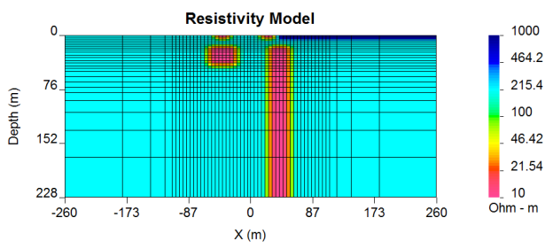
Q20: Compare your inversion models with the true model below. There are two outcropping conductors, two buried conductors and a resistive overburden. Which targets do you think are reasonably recovered by inversion? Which are not? What is the principle reason?