| |
Magnetic data used for inversion, and the predicted data based on the final 3D recovered susceptibility model are shown in this mouseover figure. Move your mouse over the image to see predicted data.
Parameters used for the 3D inversion were:
- Under the data set, the earth was discretized using rectangular cells of 25 metres x 25 metres x 12.5 metres. The model was then extended laterally outward by two large cells so that the resulting model consisted of 43 428 cells.
- The number of data was N = 1029 and errors were assigned to each datum involved as 5% of each datum value, plus a constant value of 10 nT.
- For inversion, the model objective function parameters were (m0, alphaS, alphaX, alphaY, alphaZ) = (0, 0.0005, 1.0, 1.0, 1.0).
- The reference susceptibility was assumed to be zero.
- Recovered susceptibilities were assumed to be positive.
- Topography that varies by about 100 metres over the area was included in the modeling.
- We assume that there was no remanent magnetization contributing to the observations and that demagnetization was negligible (in other words susceptibilities were assumed to be moderate).
The model objective function was standard (as discussed in all UBC-GIF tutorials on inversion), with the addition of a depth weighting function which is based upon the natural decay of dipolar magnetic fields. This is a crucial aspect of the objective function since it causes the recovered susceptibilities to be distributed with depth. Without it, the susceptibilities tend to accumulate near the surface rather than being distributed throughout the model's volume.
Resulting 3D susceptibilty model
Recovered models are 3D volumes of susceptibility. The question of how to examine the result is not trivial. Slices show values of susceptibility at all cells on the slice. Isosurface images show the shape of the susceptibility structure as a surface of constant susceptibility.
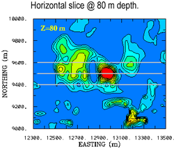
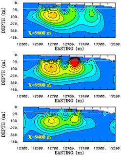
| The same information was presented in the publication on this case history using contour plots at the slices shown above. Here are colour versions of the figures in that reference (Li and Oldenburg, 1997).

|
 |
From the horizontal slice (plan section), two concentrated susceptibility highs are observed in the central region. Surrounding them are three linear anomalies trending northeast. In the cross-sections, the major anomalies are seen at moderate depth, but considerable variation in the depth to the top is evident. There are also smaller anomalies extending to the surface. In general, the models show more detailed structure near the surface and become smoother at depth.
| © UBC-GIF
January 9, 2007
|
|
|
|
|

