Geophysics foundations:    
Quick overview:  
Summary of VLF surveying and data

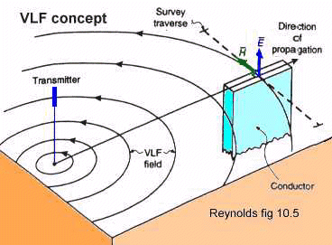
Introduction

VLF surveying involves measurement of the earth's response to EM waves generated by transmitters a great distance from the survey site. The source fields are effectively planar and of fixed orientation so the response depends on the orientation of buried objects with respect to the source fields. It is therefore usual to measure the signals caused by two or three different transmitters. Six parameters describing the secondary magnetic field are commonly measured. They are the in-phase and quadrature phase components in all three vectoral directions (x,y,z). Sometimes, the associated horizontal electric fields within the earth are also measured. This allows estimates of apparent resistivity and apparent phase between electric and magnetic fields to be recorded.

Initializing a VLF (and magnetic) instrument for a mineral exploration survey

Survey design

As for all geophysical EM surveys, the measurements respond to variations in subsurface electrical conductivity. There are several aspects that are unique to VLF surveys:

1. Owing to the fixed orientation of source fields, and to their essentially planar configuration, secondary magnetic fields are most strongly induced in long linear conductors which are oriented perpendicular to the source fields. Therefore, the response depends on target orientation as well as conductivity.
2. Large scale EM fields are capable of driving significant electric fields within the earth. These are known as galvanic currents, and they are different from the small-scale so-called "vortex" currents, which are eddy currents induced by primary magnetic fields in localized regions of higher conductivity. These galvanic currents tend to bend around regions of low conductivity. This makes it possible, under the right conditions, to detect resistive targets more easily with VLF surveys than with other shallow-investigating EM surveys.

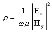
If possible, transmitters should be chosen so that the source fields they generate are perpendicular to each other at the field site. Unfortunately there are only a few transmitters around the globe, and it is difficult to survey in regions where two transmitters cannot be detected. However, when signals are present, and when only magnetic field data are recorded, acquisition proceeds nearly as fast as for an apparent conductivity or magnetic survey.

One unique aspect of the VLF technique is its ability to non-invasively record electric fields in the ground. Apparent resistivity of the ground is proportional to Ex/Hy, where Ex is electric field strength, and Hy is magnetic field strength perpendicular to the measured E-field. Acquisition of E-field data is not necessary if simple anomaly location is all that is required, but it can provide limited quantitative information on apparent resistivity and overburden thickness. Also, on sites that have very hard surface material, there is no other common method for directly measuring E-field behaviour. This is possible with VLF equipment because the frequencies involved are higher than other common geophysical methods, so capacitive ground electrodes can be used. These do not require penetration of the surface. Unfortunately, deploying the electrodes does slow down data acquisition, and results are more sensitive to ambient EM noise.

Finally, recognizing sources of noise is an important aspect of VLF survey design. For example, it is common to encounter reduced signal strength when it is drawn at the transmitter locations. Also, industrial electrical activity can be a source of noise on the data.

Raw Data

Most VLF instruments record basic electric and magnetic parameters that may be difficult to interpret directly in terms of subsurface properties. If the goal is to map the locations of buried conductors, some minor processing is recommended to emphasize conductivity structure. If the goal is to estimate depth to a target, or depth of overburden, then it is more common to plot raw data as line profiles. Both approaches are illustrated below.

Searching for buried objects with the VLF and Fraser filtered spatial maps

Figures 1-3: The buried conductive object is under location 0.0, and the transmitter is oriented off to the left side so that the source magnetic field is perpendicular to the survey line; ie in to & out of the screen. Click buttons for alternate figures. 1. Raw VLF data 2. Fraser filtering (1,1,-1,-1) 3. Both raw and filtered

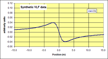
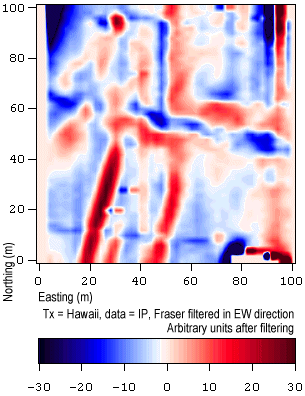
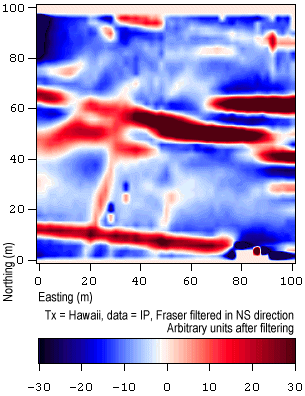
The most diagnostic parameter for locating buried conductors, especially elongated ones, is the vertical in-phase component of the secondary magnetic field. As the VLF instrument passes over the axis of a long buried conductor, this parameter's value changes sign (illustrated in Figure 1 by clicking the buttons). These cross-over positions directly identify anomaly locations on profile graphs, but maps are easier to interpret visually if cross-overs are converted into peaks using a simple filtering process described by Fraser (Figure 2 to the right). Since this is a spatial filtering technique, some smoothing will occur, and the peak's width will depend upon filter parameters, not the target's depth. Cross-overs become positive or negative peaks depending on which direction the filter is applied. Finally, cross-overs (and hence the peaks on Fraser filtered maps) will be most prominent when survey lines are perpendicular to the buried anomaly's orientation.

Once data gathered along survey lines have been Fraser filtered, results for the entire grid are contoured to identify anomaly locations. The figures below show results of Fraser filtering data sets from two different transmitters, gathered simultaneously at one site. The dependence of response on conductor orientation is immediately evident. The response is strongest if magnetic source fields are oriented perpendicular to the buried conductor because this orientation will result in the strongest possible induced currents within the buried conductor. For this reason, most modern VLF instruments record data simultaneous from two or three different transmitters (assuming, of course, that signal strength is adequate at a given site).

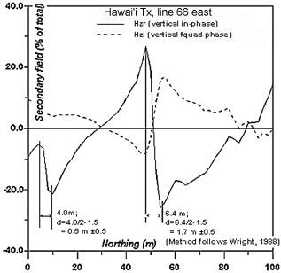Estimating depth to buried targets

For quantitative interpretation, it is more useful to plot line profiles of raw data. The figure to the right illustrates a method of estimating depth to a linear conductor based on peak to peak width of raw VLF vertical in-phase data. The depth is half the peak-to-peak width, less the instrument's elevation above ground. This procedure was developed by Wright (Wright, 1988).

Apparent resistivity

One unique aspect of VLF surveying is that horizontal electric fields in the ground can be measured using capacitively coupled electrodes. This means that the apparent resistivity can be estimated using Hx, the horizontal magnetic field measured in one direction and Ey, the electric field in the ground measured in the perpendicular direction. The relation for resistivity, ρ, is described in the following equation, where, ω is angular frequency and μ is magnetic permeability (usually μ₀):

Making E-field measurements can be a bit laborious in the field, but it may be worth the effort if apparent resistivities will contribute to the geologic question. Results are sometimes rather noisy, but depth of investigation is determined by the skin depth of the signals (around 24 kHz) rather than the geometry of transmitter/receiver systems of small apparent conductivity instruments. It is also worth noting that the presence of the buried metal affects large scale galvanic currents driven by VLF signals less than induction currents; so the apparent resistivity measured using VLF in areas where small metal features dominate induction system responses might be more reliable than apparent resistivity measured with systems that depend on induction currents.