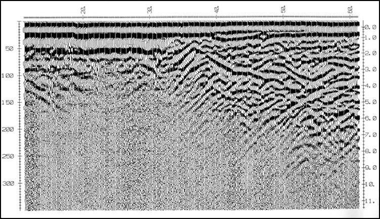
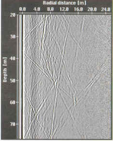
GPR can be referred to as radio echo sounding. The seismic reflection analogy is often helpful: surveying involves injecting a short pulse of energy into the ground and recording echoes. GPR energy is EM (electromagnetic - ie "radio"), therefore physical properties that affect the survey are electrical conductivity and dielectric permitivity. Results are usually presented similarly to seismic data, as position versus 2-way travel time. Wiggle trace presentation is shown here. Amplitude of the wiggle represents voltage on the antenna. More commonly the traces have one half the trace filled in (the variable area style of plot). Gray- or colour-scale images are also common, in which the colour is scaled to signal amplitude. Examples of different presentation options are given at the end of this page.
 GPR concept involving "common offset" instrument configuration. Echoes arrive from an targets that are in the range of signals. The echo surface is perpendicular to the direction of incoming signals. |
Radar data or "section" resulting from the survey shown to the left. |
 The source energy - wavelets
"Normal" radar (police speeding or traffic control systems) uses high frequency pulses and measures the power of returned energy. However, attenuation (ie absorbtion of energy) is greater for higher frequencies, and the resolution for records of returned power is limited to around a wavelength.
In order to be useful in the ground, GPR systems record voltage on antenna instead of power, thus permitting detection of the "first break" of returning pulses. Since antennas are the source of energy, it is easier to generate nearly ideal wavelets than for seismic surveys. The GPR waveform is usually a short pulse, which is therefore a wide-band signal. Bandwidth (total range of frequencies making up the wavelet) is usually ~1.5*fcenter , where fcenter is the "center" frequency determined by the antenna length.
Instruments generate short pulses by imposing a step function voltage onto an antenna. Normal dipole antennas will "ring", or oscillate. By applying resistive loading to the antenna, the emission is forced to be a short pulse rather than a continuous sinusoid (although at reduced emission energy).
Dielectric permittivity (e) and Relative dielectric permittivity (eR): explained below.
Electrical conductivity (![]() ): The second of two electrical properties affecting GPR signals in the ground. Conductivity is 1/resistivity.
): The second of two electrical properties affecting GPR signals in the ground. Conductivity is 1/resistivity.
Attenuation:
Attenuation dictates how deep we can see, and is usually described in terms of a "skin depth". Skin depth ( ![]() ) is the depth at which the field strength falls to 1/2.71828 (or 1/e) of its original amplitude. It decreases as both frequency and conductivity increase. Conductivity is the most influential parameter, as can be seen in the following table of physical properties. Maximum and minimum values (not including air, or free space) are coloured. Notice how "water" has both the highest and lowest conductivity - and hence attenuation rate - depending upon salinity. This is why the presence and composition of water is the single most significant contributor to GPR performance. Clay is also a very important factor, with only a small amount of clay contributing to significantly decreased GPR performance.
) is the depth at which the field strength falls to 1/2.71828 (or 1/e) of its original amplitude. It decreases as both frequency and conductivity increase. Conductivity is the most influential parameter, as can be seen in the following table of physical properties. Maximum and minimum values (not including air, or free space) are coloured. Notice how "water" has both the highest and lowest conductivity - and hence attenuation rate - depending upon salinity. This is why the presence and composition of water is the single most significant contributor to GPR performance. Clay is also a very important factor, with only a small amount of clay contributing to significantly decreased GPR performance.
| Table of relative dielectric permittivity (eR), electrical conductivity ( |
|||
| Material | eR |
V avg (m/ns) |
|
| Air | 1 |
0 |
.3 |
| Distilled water | 80 |
0.01 |
0.033 |
| Fresh water | 80 |
0.5 |
0.033 |
| Sea water | 80 |
3000 |
0.01 |
| Dry sand | 3- 5 |
0.01 |
0.15 |
| Saturated sand | 20-30 |
0.1-1.0 |
0.06 |
| Limestone | 4-8 |
0.5-2.0 |
0.12 |
| Shales | 5-15 |
1-100 |
0.09 |
| Silts | 5-30 |
1-100 |
0.07 |
| Clays | 5-40 |
2- 1000 |
0.06 |
| Granite | 4-6 |
0.01-1.0 |
0.13 |
| Dry salt | 5-6 |
0.01-1.0 |
0.13 |
| Ice | 3-4 |
0.01 |
0.16 |
Reflection: occurs at boundaries (where the transition zone thickness < wavelength) where ![]() or eR change. In the lossless case (i.e. when conductivity
or eR change. In the lossless case (i.e. when conductivity![]() = 0), the reflection coefficient is
= 0), the reflection coefficient is  .
.
Scattering occurs when energy is returned from features that are smaller than a wavelength. Amount of scatter is proportional to wavelength, scatterer size and material.
Spreading losses: a geometric factor; spherical losses are proportional to (range)4.
System performance: antennas, transmitter, and receiver.
Velocity: For GPR purposes we often consider only dielectric permittivity (e) to influence velocity. This is because at GPR frequencies ![]() . If e is around 10 then for omega > 106 (true for all GPR signals), sigma must be less than 105 for the condition to hold. This is often (although not always) true in earth materials. Then, assuming no magnetic materials, velocity can be approximated by
. If e is around 10 then for omega > 106 (true for all GPR signals), sigma must be less than 105 for the condition to hold. This is often (although not always) true in earth materials. Then, assuming no magnetic materials, velocity can be approximated by
where " C " is the velocity of light in air or free space, which is 300m/us. The range for velocity in typical earth materials is given in the table above. Note that a test for whether ![]() holds should be made before assuming the simple form for velocity.
holds should be made before assuming the simple form for velocity.
Dielectric permittivity (e): This physical property quantifies how easily material becomes polarized in the presence of an electric field. It is one of the two electrical properties affecting GPR signals in the ground. Somewhat counter-intuitively, free space does have a value of permittivity - it is 8.8541878176 × 10⁻¹² Farads/metre (a "Farad" is the unit of capacitance, named after Michael Faraday). If free space did not have finite permittivity, electromagnetic waves (light, radio, etc) could not propagate in free space.
Relative dielectric permittivity (eR): Relative dielectric permittivity is a ratio:
Since dielectric permittivity e=eRefree space, relative dielectric permittivity eR=e/efree space.
eR is the parameter usually referred to in GPR work. It is 1 (one) for free space or air, and 80 for water. Because it is a number that compares true value to free space value, it has no units.
Dielectric permittivity is in fact a complex value, often written ![]() , which in the notation of this page looks like er= er'+ i er". It can be considered as a measure of the extent to which charge distribution can be distorted or polarized by an applied E field.
, which in the notation of this page looks like er= er'+ i er". It can be considered as a measure of the extent to which charge distribution can be distorted or polarized by an applied E field.
The so-called "real" part (er') is the relative dielectric constant, often introduced in electronics or physics courses in the context of capacitors. It is a storage component measured as capacitance per unit length. (Capacitance is "the amount of charge a material can hold" for a given applied voltage.) At different frequencies, polarization occurs at different scales: at very high frequencies, only subatomic particles can be polarized. At GPR frequencies, re-orientation of dipolar molecules is the largest contribution, hence water's importance in determining the velocity of EM waves in a material. Note that er = 80 for water, whereas er < 10 for most other common materials.
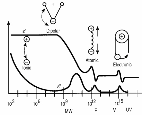
The so-called "imaginary" part (er") is a loss component that generally indicates how much energy is dissipated at the transition from one polarization mechanism to another. The behaviour of both is shown in the figure. Values are relatively constant for GPR frequencies of 106 through 109 , ensuring that wave behaviour is not dispersive; i.e. all frequency components of a broad band signal travel at the same speed.
If this discussion about dielectric permittivity seems a bit obscure, the take-home message is that the dielectric permittivity of most geological materials is closely dependant upon the amount of water (free or otherwise) in the material, and that values of er for geologic materials range from 1 to 80, as seen in the table above.
It is important to determine the velocity of radar signals in the ground because the recorded data involves time yet we want to know about depths. Velocity can be determined by measurement of GPR data in the field.
The figure below illustrate the four possible raypaths that a GPR
signal could follow. Are they all visible? Yes, under good conditions, except that the
critically refracted air wave (#4) is more than likely going to be too
weak to see. In the figure, V0
is velocity of GPR signals in air, V1 is the velocity of GPR signals in the top layer, and V2
is the velocity in the second layer.
 |
 |
In order to estimate velocity, several records must be gathered which have the same reflection point, but which involve different travel paths through the same material. Then the ambiguity resulting from having both depth and velocity unknown can be resolved. This type of survey is called a Common Mid Point (CMP) survey. A good CMP data set involves many records, and is plotted in a time-distance plot in which the trace location (horizontal axis) is a function of antenna separation, not distance along a line. For all measurements the mid point between the antennas is keeped constant. Here is a typical CMP data set. Mouseover on the figure reveals signal arrivals being discussed in the five points beneath the figure.
 It
is also possible to estimate the average velocity above a point diffractor
(such as a buried pipe, tank or boulder) using the hyperbolic diffraction from
the object (on the data plots, not the CMP). The relation is based on the T2-X2
relations for hyperbolic diffraction patterns, and is V2 = 4x2
/ (t2 - t02); parameters are defined in the
figure to the right.
It
is also possible to estimate the average velocity above a point diffractor
(such as a buried pipe, tank or boulder) using the hyperbolic diffraction from
the object (on the data plots, not the CMP). The relation is based on the T2-X2
relations for hyperbolic diffraction patterns, and is V2 = 4x2
/ (t2 - t02); parameters are defined in the
figure to the right.
 |
Left: Interactive velocity analysis using GRADIX: Below: Application of a user defined 2D velocity vs depth function to convert time-distance plots in to depth-distance.  |
There are several sources of GPR instruments. The system available for teaching at UBC is an older PulseEKKO IV system from Sensors and Software of Mississauga, Ontario. For all manufacturers, instruments basically consist of a control unit, a transmitter (Tx), and a receiver (Rx). Usually, control is managed by a laptop computer connected to the electronic control unit which converts computer initialization commands into signals for the Tx and Rx, and sends a data stream from the receiver to the computer for storage. Connections to Tx and Rx are often optical cables in order to avoid electrical and electromagnetic coupling problems. Recall that signals are in the MHz, and are of very short duration - hence very wide band.
Antennas are attached directly to the Tx and Rx, again to reduce electronic problems due to coupling and noise. There are essentially two configurations available - shielded antennas and unshielded antennas.
Examples of both types of systems, and typical data sets, are presented in figures below.
| Shielded GSSI antenna system being used for investigating
an environmental waste site.
|
 |

 |
Detection of underground storage tanks (UST's) is a common application.
|
 |
Very high frequency systems are also available for fine-scale geotechnical work. There are also a number of systems configured for towing behind a vehicle. Monitoring of railway and roadway integrity can be done very efficiently with these systems. 
|
 |
Unshielded Sensors and Software antenna system being used
for geological investigation. |
Shielded high frequency system being used to monitor mine
wall integrity in a South African mine. |
 |
GPR can also be performed for borehole investigations. This is a Sensors and software instrument.
|
This is borehole GPR data gathered using a RAMAC system
(available from Terraplus) |
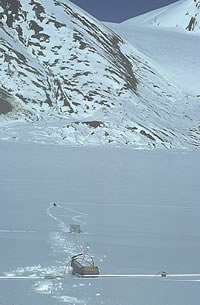
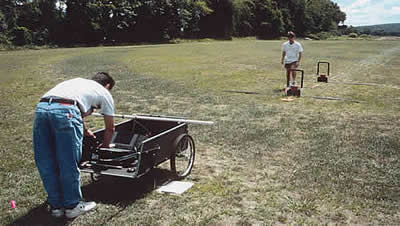
UBC students operating a Pulse Ekko GPR system with 50 Mhz antennas, investigating an acquifer in Langely, BC. |
  |
|
|

 .
.