Origin of magnetic fields
 All magnetic fields can be thought of as arising from electric currents. We are all familiar with the experiment in which a compass is held close to a wire, which can be attached to a battery. The compass needle is deflected when the current flows in the circuit. The compass itself consists of a magnet that is free to rotate. The fact that it moves indicates that the current produces a magnetic field. This was found by H. C. Oersted in 1820, and the Biot-Savart law quantifies the effect: magnetic field strength, All magnetic fields can be thought of as arising from electric currents. We are all familiar with the experiment in which a compass is held close to a wire, which can be attached to a battery. The compass needle is deflected when the current flows in the circuit. The compass itself consists of a magnet that is free to rotate. The fact that it moves indicates that the current produces a magnetic field. This was found by H. C. Oersted in 1820, and the Biot-Savart law quantifies the effect: magnetic field strength,  , at a distance, r, from a straight wire carrying current, I, in Amperes is given by the mathematical expression , at a distance, r, from a straight wire carrying current, I, in Amperes is given by the mathematical expression
 (1) (1)
The magnetic field, , is a vector. In the case of the line current, it points in a direction around the wire, given by the right hand rule. This is indicated by the unit vector,  . The units of are Am-1 (Amperes per meter). . The units of are Am-1 (Amperes per meter).
Magnetic field of a circular loop
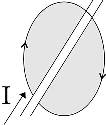
 If the current-carrying wire is bent into a loop, it produces a magnetic field with the geometry shown here. As with a straight wire, the direction of the magnetic field is given by the right hand rule. The field has the same configuration as that of a small "bar magnet" placed perpendicular to the loop's plane, at its centre. The strength of this magnetic, called m, the magnetic moment, is proportional to the current and the loop's area, A. So m=IA=I If the current-carrying wire is bent into a loop, it produces a magnetic field with the geometry shown here. As with a straight wire, the direction of the magnetic field is given by the right hand rule. The field has the same configuration as that of a small "bar magnet" placed perpendicular to the loop's plane, at its centre. The strength of this magnetic, called m, the magnetic moment, is proportional to the current and the loop's area, A. So m=IA=I r2 and has units of Am2. If the radius of the loop is a and if you observe from a distance, r, much greater than this radius (r >> a), then the strength of the field, H, decreases as 1/r3. This is a much greater rate of decrease than the 1/r we had for a long straight wire (above). r2 and has units of Am2. If the radius of the loop is a and if you observe from a distance, r, much greater than this radius (r >> a), then the strength of the field, H, decreases as 1/r3. This is a much greater rate of decrease than the 1/r we had for a long straight wire (above).
All magnetic fields are caused by currents (moving electric charges)
 We can use the relation between current loops and magnetic fields to account for any magnetic field. Consider a single atom made of protons, neutrons and electrons. Protons and electrons are charged particles which can rotate on their axes, and electrons revolve around the nucleus. One can think of these motions as "circular currents" and each circular current produces its own magnetic field. Some of the magnetic fields may cancel. For instance, electrons can have a spin up or down, but it is possible for an atom to have a net magnetic moment. This occurs especially for those atoms that have unpaired spins of the electrons. For magnetic materials, all of the magnetization that we see will be related to the cumulative effects of the magnetic moments of all of the individual atoms. In fact, the orbital motion of electrons gives rise to the diamagnetic component, and the spin motion of electrons gives rise to paramagnetic effects. We can use the relation between current loops and magnetic fields to account for any magnetic field. Consider a single atom made of protons, neutrons and electrons. Protons and electrons are charged particles which can rotate on their axes, and electrons revolve around the nucleus. One can think of these motions as "circular currents" and each circular current produces its own magnetic field. Some of the magnetic fields may cancel. For instance, electrons can have a spin up or down, but it is possible for an atom to have a net magnetic moment. This occurs especially for those atoms that have unpaired spins of the electrons. For magnetic materials, all of the magnetization that we see will be related to the cumulative effects of the magnetic moments of all of the individual atoms. In fact, the orbital motion of electrons gives rise to the diamagnetic component, and the spin motion of electrons gives rise to paramagnetic effects.
Magnetic charge and dipoles
Despite the fact that all magnetic fields have their origin in moving electric charges, it is convenient to introduce a magnetic "charge," Q, which has dimensions of Wb (Weber). Other words for Q are magnetic monopole, or pole strength. The force between two magnetic charges Qa and Qb is given by
 (2) (2)
 This is very similar to Coulomb's law, which gives the electrostatic force between to electric charges. We note that our magnetic force, F, is repulsive when the magnetic charges are the same sign ("like" poles repel) and the force is attractive when the charges have opposite sign ("unlike" poles attract). The magnetic field measurable at the location of one of the charges is the force on that charge divided by its strength, This is very similar to Coulomb's law, which gives the electrostatic force between to electric charges. We note that our magnetic force, F, is repulsive when the magnetic charges are the same sign ("like" poles repel) and the force is attractive when the charges have opposite sign ("unlike" poles attract). The magnetic field measurable at the location of one of the charges is the force on that charge divided by its strength,
 (3) (3)
In fact, the magnetic field strength, , can be thought of as the magnetic analog to the gravitational acceleration, g.
Magnetic fields of a dipole
Consider two magnetic charges of opposite magnitude (Qa = P, Qb = -P) and separated by a distance of l in free space. We refer to this configuration as a dipole. The strength of this dipolar magnet, or its magnetic moment is given by
 (4) (4)
The magnetic field away from the dipole is the superposition of the fields from the individual poles. Applying expression (3) above for the field due to both poles, we have
 (5) (5)
If r >> l then the magnetic field, , some distance away from a dipole can be found using some simple geometry. Using the polar coordiantes defined in the figure, is given by
 (6) (6)
In fact, this expression turns out to be precisely the same as that due to a circular loop current that has the same magnetic moment, but where m = IA. The similarity of fields due to a circular current loop and a magnetic dipole is emphasized in the next figure.
This correspondence has extremely important implications because it means we can think of materials as being made up of small magnets. We have substantial intuition about how small magnets act in the presence of larger magnets (everyone has put a large magnet under a sheet of paper containing iron filings). With this background, we obtain fundamental intuition about magnetic experiments. The four figures below illustrate further.
| Forces associated with magnetic monopoles |
| |
|
| Forces associated with magnetic dipoles |
| Fields due to the individual negative (yellow) and positive (blue) poles combine using vector addition into a total field shown in (purple) here, and separately to the right. |
The net field due to a dipolar source. |
| |
|
Magnetic pole strength (surface density of magnetic charge)
The anomalous magnetic field resulting from an irregularly shaped object can be accounted for using an equivalent distribution of magnetic poles on the surface of the object. Intuitive pictures can be drawn by aligning the interior magnets in the direction of the inducing field.
If the magnets point across a surface of the body, then there will be an effective pole density there. If the magnets point parallel to the interface, then the pole density will be zero.
The above not only helps with conceptualizing the character of the magnetic field, but also provides a way to calculate it directly. The magnetic field measured a distance, r, from a pole of unit strength is
 (8) (8)
where  is a unit vector pointing from the elementary pole to the observer. To find the field of the magnetized object we sum (integrate) the contributions arising from all of the poles on the surface of the body. Using the fact that is a unit vector pointing from the elementary pole to the observer. To find the field of the magnetized object we sum (integrate) the contributions arising from all of the poles on the surface of the body. Using the fact that  is the induced magnetization per unit volume (that is, = Ko ), the final field is is the induced magnetization per unit volume (that is, = Ko ), the final field is
 (9) (9)
where  is the outward-pointing normal vector to the surface. is the outward-pointing normal vector to the surface.
The anomalous field
In applied geophysics, it is common to refer to measurements as "the magnetic anomaly." This can be defined as the observed magnetic value minus a background or reference value, usually dominated by the inducing (Earth's) field. What will this anomalous field look like when total field measurements (such as those taken with a proton precession or optically pumped magnetometer) are recorded? To find out, we must analyse the combination of measurement in terms of the vector components of all contributing fields.
 Let the earth's magnetic field (really, magnetic flux) be denoted by Let the earth's magnetic field (really, magnetic flux) be denoted by  o (vertical in the figure here). Let the field from the buried magnetic feature be denoted by a. The field measured at the surface of the earth is the sum of the earth's field and the field from the buried feature. The anomalous component of that total field may be directed up or down depending upon what portion of the anomalous field is being observed (see positions A and C in the diagram). o (vertical in the figure here). Let the field from the buried magnetic feature be denoted by a. The field measured at the surface of the earth is the sum of the earth's field and the field from the buried feature. The anomalous component of that total field may be directed up or down depending upon what portion of the anomalous field is being observed (see positions A and C in the diagram).
The anomalous magnetic field that we want from a proton precession magnetometer (to be called  B) is the measured field amplitude minus the amplitude of the earth's field (which can also be called the inducing or primary field): B) is the measured field amplitude minus the amplitude of the earth's field (which can also be called the inducing or primary field):
 (10) (10)
B can usually be written in an approximate form. Let  o be a unit vector in the direction of the inducing field. In most cases |o| >> |a|. The situation can be illustrated using the following vector diagram: o be a unit vector in the direction of the inducing field. In most cases |o| >> |a|. The situation can be illustrated using the following vector diagram:
The angle q is the angle between the Earth's magnetic field and the anomalous magnetic field. Simple trigonometry tells us that
 (11) (11)
Equivalently, we can use the vector dot product to show that the anomalous field is aproximately equal to the projection of that field onto the direction of the inducing field. Using this approach we would write
 (12) (12)
This is important because, with a total field magnetometer (like a proton precession or optically pumped sensor), we can measure only that part of the anomalous field which is in the direction of the earth's main field.
Whether we work with vector component magnetometers (such as fluxgate instruments) or total field magnetometers, we are effectively able to measure only a component of the anomalous magnetic field. Here is one way to think about the measurement:
- A fluxgate oriented horizontally in the
 direction measures Bax, the projection of the anomalous field in the x-direction. direction measures Bax, the projection of the anomalous field in the x-direction.
- A fluxgate oriented vertically in the
 direction measures Baz, the projection of the anomalous field in the z-direction. direction measures Baz, the projection of the anomalous field in the z-direction.
- A total field magnetometer measures the total field. When we subtract the magnetic field of the earth to get the anomaly, then we obtain the projection of the anomalous field onto the direction of the earth's magnetic field at that location.
 |
Measured quantities
are given by:
 |
Magnetic anomaly example
| So if we know the anomalous magnetic field that arises from any magnetic body, then we also can determine what the instrument will measure. It will be the projection of the anomalous field onto the inducing field's direction. An example of the result is shown in these final three figures. Red arrows show Earth's field's direction, blue arrows show induced field vectors, and the sign of measurements can be determined by comparing the directions of these two fields at each location on the earth's surface.
On a piece of paper, sketch a blank version of the empty graph; then try to sketch qualitatively the measurement you would expect along the surface. For example, at the equator (Figure 1) the largest measurement will be above the centre of the buried object, and it will have negative magnitude because the object's field points in the opposite direction to the earth's field. Confirm your sketches using the "Solution" buttons.
|
 |
|