| |
This is a short tutorial on how to invert a small set of magnetic data with MAG3D.
Installing educational versions of codes
- RIGHT-Click this link here, and save this self-contained install program to a convenient place on your computer (for example, the desktop).
- Then run this installation program, and follow instructions for reading the License, and specifying installation folders.
- After this installation, you can delete the Install Program saved at step 1.
 Generate a simple magnetic data set Generate a simple magnetic data set
Run the MeshTools3D program (from the Start menu, or by double clicking the MeshTools3d.exe file).
- Read the banner text, then click "OK".
- Ignore the initial dialogue by clicking "Cancel".
- Define a volume by selecting "File => Create mesh ...".
- Change nothing - just save this mesh as follows:
- Click the save button - IMPORTANT: find the "first-test" subfolder within the folder where programs were put.
- Change to that folder
- Enter "mesh1.txt" as the filename, then click the "Save" button.
- You should see the blank volume in the MeshTools3D window.
- Add a density anomlay in this volume as follows:
- Select "Edit => Add blocks ... " and click "yes".
- Do not change anything in the "Add Blocks dialogue, EXCEPT to make "Value" = 0.1, and the Z-coordinates = -10, -20 (next to the set button). (Units for these parameters are S.I. units of susceptibility, and metres respectively.)
- Click the "set" button.
- Click the "OK" button.
- Save this model in the same place as the mesh using the "File => Save as ..." option. Call this model "model1.txt".
- Now calculate magnetic data over this model (forward modelling) as follows:
- Select "Forward model => Magnetics ".
- None of the parameters in this dialogue need to be changed for a first trial - just click "OK".
- Aside: If you want to generate magnetic data that would be observed at a particular location on Earth, you need to set Inclination, Declination, and Field strength so they are compatible with Earth's magnetic field at that location. For example, at Vancouver, British Columbia, Canada, these values are (I,D,F)=(72,27,56,000); i.e., inclination is 72 degrees down from horizontal, declination is 27 degrees right of north, and field strength is 56,000 nano Teslas (nT).
- If you do not change parameters in this dialogue you are calculating data as if you were at the equator, at a location where magnetic north is in line with true north, and Earth's field has a strength of 44,000 nT.
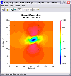
- You will be shown two banners each with an "OK" button - click these to obtain the data set displayed in a gm-data-viewer window.
- You have just forward modelled a simple synthetic scenario. The resulting magnetic data over our volume with it's small magnetically susceptible anomaly is shown in the figure above right.
- See the MeshTools3D program's user manual for details about using this program for generating 3D models and forward modelling gravity or magnetic data.
NOTE: If this synthetic data set was to be inverted, you would have to add noise to the data. See the gm-data-viewer manual for instructions. For this quickstart, you do NOT have to do anything because the noisy data set is provided.
 Invert this simple data set Invert this simple data set
Close the MeshTools3D and gm-data-viewer programs.
Run the MAG3D's graphical user interface (GUI) program from the Start menu (or by double clicking the mag3d-gui.exe file).
- Read the banner that pops up, then click OK.
- The "Mag Observation File" dialogue appears; click the Browse button to find the data file called "magdata-noisy.txt" in the first-test folder (under the program's folder).
- Click the "View Data / Errors" button to see this data set.
- In this data viewing window, display standard deviations that were assigned by selecting "View => Errors" (or clicking the "errors" toolbar button), then close the data viewing window.
- Click the "Create mesh" button in order to build a mesh suitable for discretizing the volume of ground under the data set (remember, the inversion program doesn't know this is synthetic data that you created).
- In the Create mesh dialogue, enter 15 for "Width of cells", then click "Save". Call this mesh file "inversion-mesh.txt".
- Now save all default parameters for the first inversion as follows:
- Select "File => Save" (or click the "save" toolbar button).
- Browse to the "first-test" sub-folder.
- Click "Save" (leave the default filenames as is).
- The "Run" toolbar button should now be active (with a green underline). Click it to start the inversion.
- A command line window should pop up, displaying each step in the inversion's iterative process. The inversion should take several seconds for this tiny problem.
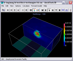
- When it is finished, view the resulting model by selecting "View => Model" (or by clicking the "model" toolbar button).
The model of magnetic susceptibility contrast within the ground under the synthetic magnetic data, produced by this inversion, is shown in the figure to the right.
- (There may be susceptible zones within the padding cells of the model (large cells added around the region of interest). Usually this occurs when the area covered by data is not large enough for signal caused by buried susceptible zones to have decayed fully to zero. Observe your data set and see if values around survey area edges is NOT zero - like the data set illustrated above. )
- See the MeshTools3D program's user manual for details of using this program for viewing 3D models.
- No inversion result should be used without carrying out appropriate quality assessment steps, and without generating several alternative models. See the program manuals (IAG Chapter 10) or the mag3d/grav3d workflow for details (IAG's Chapter 7).
That's it. You have completed your first inversion of magnetic data.
Please see the MAG3D subsection of the "Sftwr & manuals" menu of IAG to find the Workflow, and the MAG3D manual for details about carrying out effective inversions, and using the tools available.
FINALLY:
- REMEMBER THAT INVERSION PROCESSING IS NOT TRIVIAL.
- LEARN ABOUT HOW IT WORKS BEFORE USING RESULTS TO MAKE IMPORTANT DECISIONS. |
|
