Exercise 2 - Calculation of Vertical Dynamic Ocean Modes
Based on https://github.com/sea-mat/dynmodes/blob/master/dynmodes.m by John Klinck, 1999.
The goal is to calculate and explore the vertical dynamic modes using a Python function that calculates numerical solutions of the generalized eigenvalue problem expressed by:
(1)¶\[\frac{\partial^2}{\partial z^2} w_m + \alpha^2 N^2 w_m = 0\]
with boundary conditions of \(w_m = 0\) at the surface and the bottom.
Variables:
\(z\) is the vertical coordinate, measured in \([m]\)
\(w_m\) are the vertical velocity modes
\(N^2\) is a profile of Brunt-Vaisala (buoyancy) frequencies squared \([s^{-2}]\)
\(\alpha^2\) are the eigenvalues
Your assignment:
Get the Python Code
Open up a terminal window and an editor,
and go to the dynmodes directory.
Please see the Get the Python Code section in Exercise 1 if you haven’t already cloned the AIMS-Workshop repository from GitHub.
Change to the AIMS-Workshop/dynmodes/ directory and start ipython with plotting enabled.
The Python functions we’re going to use in this exercise are in dynmodes.py.
The dynmodes() Function
The dynmodes() function has the following docstring that tells us about what it does,
its inputs,
and its outputs:
- dynmodes.dynmodes(Nsq, depth, nmodes)[source]
Calculate the 1st nmodes ocean dynamic vertical modes given a profile of Brunt-Vaisala (buoyancy) frequencies squared.
Based on https://github.com/sea-mat/dynmodes/blob/master/dynmodes.m by John Klinck, 1999.
- Parameters:
Nsq (
numpy.ndarray) – Brunt-Vaisala (buoyancy) frequencies squared in [1/s^2]depth (
numpy.ndarray) – Depths in [m]nmodes (int) – Number of modes to calculate
- Returns:
(wmodes, pmodes, rmodes, ce)vertical velocity modes, horizontal velocity modes, vertical density modes, modal speeds- Return type:
tuple of
numpy.ndarray
Analytical Test Cases
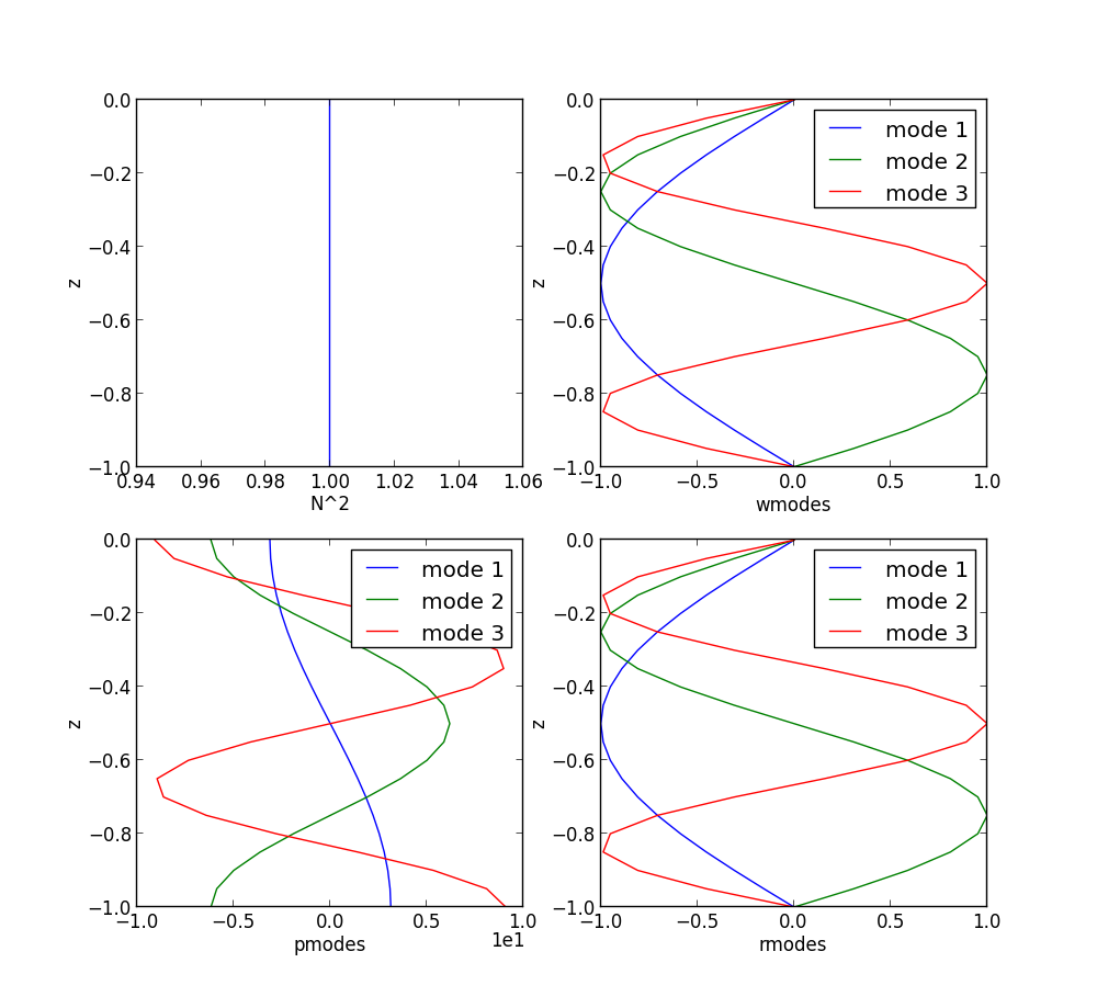
For unit depth and uniform, unit \(N^2\) the analytical solution of the (1) is:
where
and \(w_o\) is an arbitrary constant, taken as 1.
Calculate the 1st 3 dynamic modes for this case using dynmodes():
In []: import numpy as np

In []: import dynmodes

In []: depth = np.linspace(0, 1, 21)

In []: Nsq = np.ones_like(depth)

In []: wmodes, pmodes, rmodes, ce = dynmodes.dynmodes(Nsq, depth, 3)

In []: ce
Out[]: array([ 0.31863737,  0.15981133,  0.10709144])
Calculate the 1st 3 modes of the analytical solution for this case:
In []: const = 1 / np.pi

In []: analytical = np.array((const, const / 2, const / 3))

In []: analytical
Out[]: array([ 0.31830989,  0.15915494,  0.1061033 ])
Finally, plot \(N^2\) and the vertical and horizontal modes, and the vertical density modes:
In []: dynmodes.plot_modes(Nsq, depth, 3, wmodes, pmodes, rmodes)
Another case with an analytical solution that you can try is:
400 \(m\) depth at 10 \(m\) intervals
Uniform \(N^2 = 1 \times 10^{-6} \ s^{-2}\)
The analytical solution is:
where
Exploring Different Stratifications
There are 4 density profile files for you to explore:
SoG_S3.densis from the Strait of Georgia on the west coast of Canadas105.densands109.densare from Florida Straitsso550.densis from the South Atlantic offshore of Cape Town
The dynmodes.read_density_profile() function will read those files and return depth and density arrays.
You can view its docstring via the ipython help feature:
In []: dynmodes.read_density_profile?
The dynmodes.density2Nsq() function will convert a density profile to a profile of Brunt-Vaisala (buoyancy) frequencies squared.