b) Read the 2021 BC Primer on Air Quality Modeling. https://www2.gov.bc.ca/assets/gov/environment/air-land-water/air/reports-pub/primer_bc_dispersion_modelling_guideline_2021.pdf
Do in-class exercise of creating an updated table of concentrations for air quality standards in different countries.
b) Skim the 2022 BC Modeling Guideline. https://www2.gov.bc.ca/assets/gov/environment/air-land-water/air/reports-pub/bc_dispersion_modelling_guideline.pdf
a) Read Chapter 5 Atmospheric Stability from Stull, 2017: Practical Meteorology.
b) Reinforce your understanding by reading p1 - 37 from the BC MoE 2017 talk.
c) Get an account on the EOAS dept computer cluster called "optimum".
Do the exercise (as described in detail in Piazza) to determine static and dynamic stability, and height ranges of turbulent air, based on the attached sounding. We will discuss your answers in class on Wed 17 Jan 2024 in class.
# Gaussian Plume - simple
# R. Stull, 8 Feb 2016, Modified 4 Jul 2018 & 10 Jan 2024.
# Givens ==============
# meteorology
m = 20. # wind speed (m/s)
zi = 2000. # mixed layer depth (m)
sigma_v = 1.3 # lateral velocity standard deviation (m/s)
sigma_w = 1.02 # vertical velocity standard deviation (m/s)
tl = 60. # Lagrangian time scale (s)
# plume
zcl = 150. # plume centerline height (m)
q = 300. # emission rate (g/s)
# domain, assuming origin (x, y, z) = (0,0,0) is a base of smoke stack
xmax = 10000. # x downwind domain size for x = 0 to xmax (m)
ymax = 500. # y crosswind domain size for y = -ymax to +ymax (m)
zmax = 500. # z vertical domain size for z = 0 to zmax (m)
# spatial resolution for calculations of concentration
delx = 200. # x increment (m)
dely = 20. # y increment (m)
delz = 20. # z increment(m)
# Assignment ==============
# Create contour plots of concentration (µg/m^3)
# using Stull eq.(19.20) with eqs. (19.13) within the domain for:
# a) horizontal (x,y) slice at earth's surface (z = 0)
# b) horizontal (x,y) slice at height of plume centerline (z = zcl).
# c) vertical along-wind (x,z) slice of thru plume centerline (y = 0)
# d) vertical crosswind (y,z) slices at two downwind distances x
# from the stack of
xslice1 = 2000. # x-location of crosswind (y,z) slice (m)
xslice2 = 5000. # x-location of crosswind (y,z) slice (m)
# Hints:
# Use any computer language; e.g., R, MatLab, python, fortran, excel. (I used R.)
# Use a contour interval of 20 µg/m^3.
# Check that your answer to part (a) is similar to the sample
# application (Solved Example) in Stull p734 before you do the
# other parts. (It won't be exactly equal, because of different
# inputs in this HW assignment.)
# Turn in your contour plots AND your code.
# Please have your name on everything you turn in.
#
You can write your code in any language; e.g., R, MatLab, python, fortran, excel, etc. Due on 24 January 2024 (submit your code and results and plots via Canvas).
(Note, although the assignment description at left is written using syntax for the R language, you may use any computer language you want. In R, the # symbol denotes the start of a comment.)
Install AERMOD on the "optimum" computer, and run the test case. See details at https://www.eoas.ubc.ca/courses/atsc507/ADM/aermod/index.html
-and-
Install AERMET on "optimum", and run the test case. See details at https://www.eoas.ubc.ca/courses/atsc507/ADM/aermod/index.html .
-and-
Install AERMAP on optimum, and run test case. See details at https://www.eoas.ubc.ca/courses/atsc507/ADM/aermod/index.html .
Present a section of the AERMOD Model Formulation material to the class.
a) Look over the EPA AERMOD home page
https://www.epa.gov/scram/air-quality-dispersion-modeling-preferred-and-recommended-models#aermod
b) 2023 AERMOD Model Formulation document https://gaftp.epa.gov/Air/aqmg/SCRAM/models/preferred/aermod/aermod_mfd.pdf
Use Piazza to communicate with me and other students to decide who wants to present which
section, so that there are no duplicate presentations. One topic
per student. Your topic choices are:
- Energy Balance. p 19-22.
- Derived Parameters in Convective Boundary Layer (CBL). p 22-24 .
- Derived Parameters in the Stable Boundary Layer (SBL). p 24-30.
- Mixing height & adjustment for low wind. p 30 - 35.
- Wind and temperature profiling. p 36-42
- Vertical, lateral, and mechanical turbulence. p 42-50.
- Vertical inhomogeneity in the boundary layer. p 51-56
- General structure of AERMOD including terrain. p 57-65.
- Concentration predictions in the CBL. p 66-75.
- Gaussian plume eqs for direct, indirect, & penetrated sources in CBL. p 75-78.
- Gaussian plume in SBL including meander. p 79-83.
- Estimation of sigma_y and sigma_z. p 83-93.
- Plume rise. p 93-98
- Other topics including plume volume method. p 99-105
- Urban boundary layer. p105-111.
Finish student presentations (see above).
Everyone, please go to the Hysplit page and register. It is free, but there could be a week delay between when you register and when you have access to the hysplit source code. So by starting now, you will be ready for the hysplit lessons in a couple weeks.
https://www.ready.noaa.gov/HYSPLIT_register.php
Also, Stull will lecture on:
- Plume rise theory
- Lagrangian particle dispersion (in preparation for hysplit)
Stull continues lecture on Lagrangian particle dispersion.
Write code for the following exercise:
# Deardorff Plume Dispersion in Unstable PBL
# R. Stull, 13 Feb 2016, and 27 Feb 2024
# Re-read Stull (2017) Practical Meteorology, Chapter 19, pages 735-738.
# Givens ==============
# meteorology
g_by_tv = 0.0333 # g/Tv approx. constant (m s^-2 K^-1)
mycase = c("Morning", "Mid-day") # To identify each case
m = c(2., 5.) # wind speed (m/s) in (morning , mid-day)
zi = c(100., 1000.) # mixed layer depth (m) in (morning , mid-day)
FH = c(0.05, 0.2) # effective surface kinematic heat flux (K m/s) in (morning , mid-day)
# plume
zs = 75. # source height of pollutants after plume rise (m)
q = 300. # emission rate (g/s)
xmax_d = 6. # dimensionless max distance X downwind, for Deardorff's calculations
ymax_d = 5. # dimensionless max crosswind range, for Y within +- ymax_d.
# Assignment ==============
# Use any computer language; e.g., R, matlab, python, fortran, excel. (I used R.)
# (A) Plot the dimensionless Zcl vs. X curves (analogous to Stull Fig. 19.7), with separate curves
# for the two cases (morning, midday).
# Hint: Increment X between 0 and 6 (using very small delta-X at small X,
# and larger deltz-X as X gets larger),
# and apply to eq. (19.32). Use 0 ≤ Zcl ≤ 1 for the range of dimensionless heights on the
# vertical axis of the graph
.
# (B) Find and plot the dimensionless cross-wind integrated concentration contours
# (similar to Stull Fig. 19.8),
# but for dimensionless release heights corresponding to the two cases (morning , mid-day),
# for dimensionless ranges: 0 ≤ X ≤ 6 and 0 ≤ Z ≤ 1 .
# ==> Tips on how to do this are from the Practical Meteorology "Errata" link, copied here:
#
1) eq. (19.33) indicates that Cy' is a function of dimensionless height Z and dimensionless
# downwind distance X (via eq. 19.34 and eq. 19.32).
# Thus, Cy' is a 2-D array: Cy' (X, Z) which you will use in the next step.
# 2) eq (19.35) should indicate that for any one column in the matrix (i.e., for any fixed X),
# sum Cy' over all heights Z for that one X to find the average Cybar (X) .
# 3) then eq (19.36) implies for that same fixed X, divide each element (i.e., for each height) in
# that one column of Cy' by its average Cybar (X), to give the desired Cy (X, Z) for that one X.
# 4) Repeat the previous 2 steps separately for each X. After finishing those operations, you now
# have the properly-scaled new 2-D matrix Cy (X, Z), such as was plotted in Fig. 19.8.
# (C) For the range of for 0 ≤ X ≤ 6 and 0 ≤ Cy ≤ 4 , Plot a graph of dimensionless
# Cy vs. X, at Z =0, with separate curves for each of the two cases.
# Namely, this is the dimensionless crosswind integrated concentration at the ground,
# vs. dimensionless downwind distance X.
# Confirm that these curves agree with the
# the concentration values from your contour plots from (B).
# (D) Create contour plots of the dimensionless concentration C at the earth's surface (Z = 0), for
# a surface map spanning the following region: dimensionless coordinates of 0 ≤ X ≤ 6 and -5 ≤ Y ≤ 5 ,
# using a separate plot for each case (morning, midday).
# Plot the concentration isopleths for dimensionless C values of
# levels = c( seq(0.05, 0.35, 0.05) , seq(0.4, 2.0, 0.2), seq(3, 10, 1) ),
# [ where in R, the sequence command gives evenly-spaced values with
# seq(starting value , ending value , increment) .]
# Note: this exercise can be built on your results from exercise (B).
# (E) Same as D, but plot contours for actual concentrations c (mg/m3) vs. actual distances x (m) and y (m).
# Hints: Your plot domain could be for 0 ≤ x ≤ 2,500 m , and -500 ≤ y ≤ 500 m .
# You can draw the concentration contours for the following values:
# c (mg/m3) = 0.01, 0.05, 0.1, 0.2, 0.3, 0.5, 1.0 , 2.0 , 3.0 , 5.0 , 10.0 , 15.0, 20.0 , 30.0
# (F) Plot a graph of actual ground-level (z=0) centerline (y=0) concentration c (mg/m3) as a function
# of actual distance x (m) downwind, for 0 ≤ x ≤ 3,000 m,
# for concentrations in the range 0 ≤ c ≤ 20. (mg/m3).
# On the one graph, use separate curves for each case (morning, midday), but with the same x axis.
# Namely, this is similar exercise (C), but with real values instead of dimensionless values.
# Check that these curves agree with your figures from exercise (E).
# (G) Discuss:
# (1) Why does C or c decrease seemingly monotonically with increasing distance X or x
# downwind of the first maximum, even though
# the crosswind-integrated concentrations Cy of exercises (B) or (C) seem to show
# a secondary relative minimum at distances of roughly X = 1.5 to 2.5 (dimensionless)
# with a secondary relative maximum beyond that ?
# (2) Why do the morning and mid-day cases give the max concentrations at roughly the same
# real x (m) location downwind, even though the cross-wind integrated
# concentrations for the mid-day case
# bring the high concentrations down to the surface much sooner than for the morning case?
# (3) Given your contour plots from exercise (E), what is the primary advantage of using this
# convective dispersion method (i.e., Deardorff, as approximated by Stull) over using a traditional
# Gaussian plume?
# Check your answers and discuss the significance.
# Turn in your code and the contour plots as a unified pdf plot, such as a pdf printout from a Jupyter notebook.
This
is a chance for you to learn about dispersion in a convective
(statically unstable) boundary layer - - also known as a mixed
layer. It uses the discoveries by Deardoff and Willis, as
parameterized by me in my Practical Meteorology book.
Read and follow the instructions in the order given - - it will gently
lead you towards a better understanding of dispersion in a convective
pbl.
You can write your code in any language; e.g., R, MatLab, python, fortran, excel, etc.
Due 7 Feb 2024.
The following is NOT assigned for the 2024 course. So ignore the info below.
Due today is your run of AERMOD (and AIRMET and AIRMAP if needed) for a somewhat actual case:
Battle River Generating Station
Alberta, Canada
about 150 km southeast of Edmonton, AB.
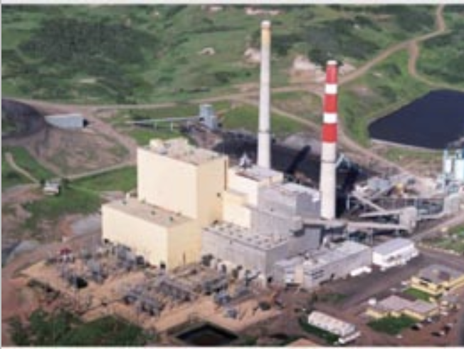
Stack C (Unit 5)
height of stack-top above ground: 161 m
diameter of stack: 5.8 m
fuel: coal
SO2 emission rate: 22,961 tonnes/year
Run your AERMOD for one year only. (You can pick the year, based on data availability.)
Upper air data: Edmonton Stony Plain.
Need to use only the morning (12 UTC) soundings.
Select "Mandatory AND Significant Levels".
Station identifier: WSE
- WMO Station number: 71119
- Observation time: 180714/0000
- Station latitude: 53.53
- Station longitude: -114.10
- Station elevation above sea level (m): 766.0
Surface weather data. Nearby weather stations are: Coronation, or Red Deer, or Edmonton, AB.
Note: if you are unable to find a surface data archive in the correct format for a Canadian station near Battle River, then for the purpose of this learning-exercise, use Havre City-County Airport (KHVR) in Havre, Montana, USA. It is roughly the same distance east of the Rocky Mtns ad Battle River.
Lat: 48.54278°NLon: 109.76333°WElev: 2589ft. , and pretend it is at Battle River. WMO Id: 72777.
For roughness length, albedo, and Bowen ratio, use Google Maps street view to see the local surface near the power plant. (Hint you can see the smokestacks in the distance from the road, if you look in the right direction.) In your submitted report, justify your choice of these 3 variables.
For tips on doing this, see the AERMOD implementation guide. https://www3.epa.gov/ttn/scram/models/aermod/aermod_implementation_guide.pdf
But for this learning-exercise, pretend the surrounding terrain is flat, and that all receptors are at the same elevation as the base of the smokestack.
Put receptors on a cartesian grid, with 2 km grid spacing extending 50 km from the smokestack in each of the main compass directions (north, east, south, west).
In addition to turning in the AERMOD output, please create a 1-page summary/overview report, and indicate which receptor locations (if any) exceed the Canadian air-quality standards for SO2.
(Please see me if you need additional info or have questions for this exercise.)
.
.