Finite-difference Methods - Spatial & Temporal

Under construction (this web page, and most other web pages for this course).

Instructor: Roland Stull

A. Spatial Differencing

Learning Goals:   By the end of this module, you will be able to ...

• draw Arakawa staggered grids A - E.
• use Taylors series to derive second-order accurate finite spatial-difference approximations for first through 4th-derivatives.
• derive finite-difference approximations of any truncation accuracy up to 4th order.
• list the grid computation rules for staggered grids.
• explain the role of stencils in aligning physical variables over appropriate grid points for operations (addition and multiplication) for staggered grids. 

Readings BEFORE class:

1. Stull p752-758, and
2. Warner  p17-23 & p51-58 on time- and space-differencing. 

Homework AFTER class:

1. Catch up on all previous readings.
   

Topics

A. Grid Points,   Grid Cells,  &  Staggered Grids.

1. Arakawa A thru Arakawa E grids

B. Spatial-gradient Differencing

1. some finite difference approximations for 1st, 2nd, and 3rd derivatives
2. approximations at various truncation orders.
3. stencils

B. Temporal Differencing

Learning Goals:   By the end of this module, you will be able to ...

• write the finite-difference approximations for named time-differencing schemes.
• explain graphically how higher-order schemes step forward in time.
• discuss the Runge-Kutta 3rd order scheme used in the WRF model.
• [Possibly: write your own simple forecast model with appropriate spatial and temporal differencing schemes.]

Readings BEFORE class:

1. read: Warner p58-72.

Homework AFTER class:

1. Do Homework #4 :   
   Given the following description of the actual temperature (T) field and its variation with time (t):
   
   T(°C) =A * (c*t + T_ref - T_{ref_o}) * (T_{ref_o} - c*t)
   
   with :

• T_{ref_o} = 2 ,     is a fudge factor
• A = 1,    is arbitrary amplitude
• c = 1.5,    is a fudge factor to make an interesting looking temperature field
• ∆t = 1   is the time step, 
• t = m*∆t   is time,
• m = time-step index
  [Note: This function was the basis for the worksheet that I handed out in class (the coloured curved lines in the fig below), where I used variable T_ref in the range of 2 to 6, and m in the range of 0 to 1. Different T_ref values give the different curves in the figure, and T_ref is constant along any one curve.]
  

Since the temperature equation above is a function of both time and temperature, I've calculated the temperature tendency for you. Namely, the slope of the lines at any point in the figure:

∂T/∂t = f(t, T) = 1.5 * { 2 – 1.5*t – [ T / (2 – 1.5*t) ] }

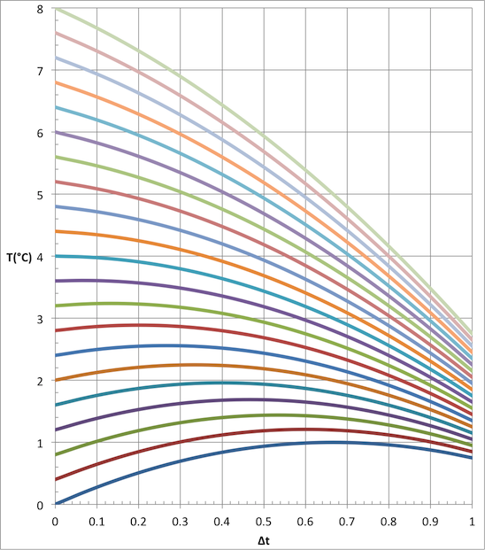
[Note: To get the eq above for f(t, T), I first solved the original temperature-field eq for T_ref(T, t).  Then I  analytically found ∂T/∂t from the first equation above, and substituted in the expression for T_ref.  This takes advantage of the fact that T_ref is constant along any of the curves in the fig below.]

.


.
Given the temperature-field and temperature-tendency info above, and given the initial condition below, apply finite difference methods (a) - (d) to predict the temperature after 1 full timestep ahead. Namely:

Please start from initial condition of T = 2 degC at m = 0, as we did in class, but compute using any programming language (excel, matlab, R, python, fortran, etc) the new T (degC) at 1 timestep (1∆t) ahead using:
a) Euler forward
b) RK2
c) RK3
d) RK4
e) Which one gave an answer closest to the actual analytical answer as given by the function above?   [Note: do NOT use the 1-D model from the previous HW for this.]

Topics

A. Named Finite-Difference Schemes.

1. Euler forward & backward,
2. Leapfrog,
3. Runge-Kutta (2nd, 3rd, and 4th order),
4. Adams-Bashforth,
5. Predictor-corrector (Lax Wendroff, Matsuno, etc.)
6. [Perhaps others]