| |
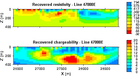
The 177 data points presented as pseudosections in the pre-processing section were inverted using the algorithm described in Oldenburg and Li (1994). The 2D section under the survey line was divided into 2000 rectangular cells, each having a constant resistivity and chargeability. First the DC resistivity data were inverted. Data were assigned a 3% error and a model objective function was specified so that the recovered model would be equally smooth in horizontal and vertical directions, and a reference model of 10 Ohm-m was used. In other words, the result would tend to revert to the refrence model value in regions where the data did not constrain the model. The inversion process was nonlinear and iterations were required. The variable for the inversion was log of resistivity. The recovered model is shown in the top panel Figure 2.
 Figure 2
. Inverted sections of resisitivity (top) and chargeability (bottom). Colour scales have the same units as Figure 1 (Ohm-m and milliradians), but the vertical scale is now in meters. |
The recovered resistivity model was used to calculate the sensitivity matrix for inversion of the IP data. The model discretization for IP inversion was the same as for DC resistivity. The reference model was zero, and data were assigned an error of 0.5 mrad. The variable for inversion was chargeability (in mrad, the same units as the data), and the recovered model is shown below that of the resistivity model in Figure 2.
 home © UBC-GIF
April 23, 2007 home © UBC-GIF
April 23, 2007
|
|
|
|
|

