|
DCIP2D:
|
|
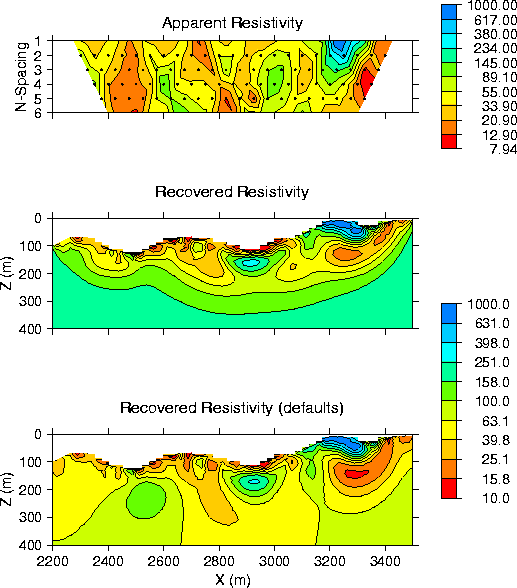
Previous Page (Fine-mesh Inversion) As a field data example, we consider a data set supplied by Newmont Gold Company. The data were acquired using dipole-dipole arrays having a=50 m and n=1, 6. A total of 127 observations were collected for both DC and IP experiments. There is strong topographic relief present along the traverse. This data set was used in the JACI Technical Note TN005 to illustrate the inclusion of topography in DCIP2D Version 2.0 and the inversion results have been shown to be consistent with geology. In this section, we re-invert the data set using DCIP2D Version 3.0 and illustrate the performance of the default mode in the inversion programs. DC Inversions The apparent
resistivity pseudo-section is shown in the top panel. For the original
inversions, we have assigned to the DC potentials an error standard
deviation that is equal to 5% of the datum magnitude plus a minimum of
0.1 mV. The inversion is able to fit the data to a We have inverted the data again using Version 3.0 by supplying only the data and surface topography and setting the remaining input to their default values. The resultant model is shown in the bottom panel. The two models are consistent with each other and show many common features. The major difference occurs towards the bottom of the models due to the different reference models used in the inversion.
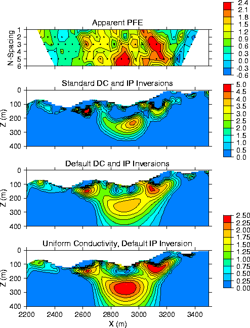
IP Inversions The apparent PFE pseudo-section is shown in the top panel.
For the original inversion, we have assigned an error standard deviation
that is 5% of each datum plus a minimum of 0.1. The inversion fits the
data to a We next carry out the IP inversion using the default mesh and the conductivity model from the default DC inversion. Default data errors are assigned by the program. The resultant model is shown in the third panel. This model has a much lower amplitude than the standard inversion and it appears to be smoother. However, it shows three anomalies of variable size as does the model from the standard IP inversion. The locations of the anomalies are also consistent between the two models. Finally, the IP data are also inverted using all possible default parameters, which means that the inversion uses the sensitivity from a uniform halfspace conductivity. This inversion then differs from the preceding one only in the conductivity model used for calculating sensitivity. The resultant model is shown in the bottom panel and it is similar to the one in the third panel. The deep chargeable body has a higher amplitude. Overall, the default mode of the inversion program has performed satisfactorily.
|
 value of 75. The
resultant model is shown in the middle panel.
value of 75. The
resultant model is shown in the middle panel.