|
Next Page (Forward Modelling)
Introduction
This manual presents theoretical background, numerical examples, and
explanation for implementing the program library DCIP2D. This suite of
algorithms, developed at the UBC-Geophysical Inversion Facility, are
needed to invert DC potentials and IP responses over a 2-D earth
structure. The manual is designed so that a geophysicist who has an
understanding about DC resistivity and Induced Polarization field
experiments, but who is not necessarily versed in the details of inverse
theory, can use the codes and invert his or her data.
A typical DC/IP experiment involves inputting a current I to the ground
and measuring the potential away from the source. In a time-domain
system the current has a duty cycle which alternates the direction of
the current and has off-times between the current pulses at which the IP
voltages are measured. A typical time-domain signature is shown in Fig.
1. In that Figure,  is the potential that is measured in
the absence of chargeability effects. This is the "instantaneous" value
of the potential measured when the current is turned on. In mathematical
terms this potential is related to the electrical conductivity is the potential that is measured in
the absence of chargeability effects. This is the "instantaneous" value
of the potential measured when the current is turned on. In mathematical
terms this potential is related to the electrical conductivity  by by
 (1) (1)
where the forward mapping operator  is defined by the equation is defined by the equation
 (2) (2)
and appropriate boundary conditions. In equation (2) is the
electrical conductivity in Siemen/metre (S/m),  is the gradient
operator, I is the strength of the input current in Amperes, and rs is the
location of the current source. For typical earth structures ,
while positive, can vary over many orders of magnitude.
The potential in equation (2) is the potential
due to a single current. This is the value
that would be measured in a pole-pole experiment. If potentials from
pole-dipole or dipole-dipole surveys are to be generated then they can
be obtained by using equation (2) and the principle of superposition. is the gradient
operator, I is the strength of the input current in Amperes, and rs is the
location of the current source. For typical earth structures ,
while positive, can vary over many orders of magnitude.
The potential in equation (2) is the potential
due to a single current. This is the value
that would be measured in a pole-pole experiment. If potentials from
pole-dipole or dipole-dipole surveys are to be generated then they can
be obtained by using equation (2) and the principle of superposition.
When the earth material is chargeable the measured voltage will change
with time and reach a limit value which is denoted by  in
Fig. 1. There are a multitude of microscopic polarization phenomena
which collaborate so that this final value is achieved but all of these
effects can be consolidated into a single macroscopic parameter called
"chargeability". We denote chargeability by the symbol in
Fig. 1. There are a multitude of microscopic polarization phenomena
which collaborate so that this final value is achieved but all of these
effects can be consolidated into a single macroscopic parameter called
"chargeability". We denote chargeability by the symbol  . Chargeability is dimensionless, positive, and confined to the region [0,1). . Chargeability is dimensionless, positive, and confined to the region [0,1).
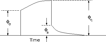
Figure 1 Definition of the three potentials associated with DC/IP experiments.
To carry out forward modelling to compute we adopt Siegel's
(1959) formulation which says that the effect of a chargeable ground is
modelled by using the dc resistivity forward mapping but with the
conductivity replaced by  . Thus . Thus
 (3 (3
or
 (4) (4)
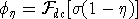
The IP datum, which we refer to as apparent chargeability, is defined by
 (5 (5
or
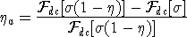 (6 (6
Equation (6) shows that the apparent chargeability can be computed by
carrying out two DC resistivity forward modellings with conductivities
and (1- ) . Note that in this definition apparent
chargeability is dimensionless and, in the case of data acquired over an
earth having constant chargeability 0 , we have a = 0 .
The field data from a DC/IP survey are a set of N potentials (ideally
but usually ) and a set of N secondary
potentials  or a quantity that is related to . The goal of
the inversionist is to use these data to acquire quantitative
information about the distribution of the two physical parameters of
interest: conductivity (x,y,z) and chargeability (x,y,z) . or a quantity that is related to . The goal of
the inversionist is to use these data to acquire quantitative
information about the distribution of the two physical parameters of
interest: conductivity (x,y,z) and chargeability (x,y,z) .
The distribution of conductivity and chargeability in the earth can be
extremely complicated. Assuredly earth structure is 3D but for the DC/IP
codes developed here we restrict ourselves to 2D structures and assume
that the survey has been carried out along a traverse which is
perpendicular to strike. The cross-section of the earth is divided into
rectangular prisms each having a constant value of conductivity and
chargeability.
Next Page (Forward Modelling)
|
