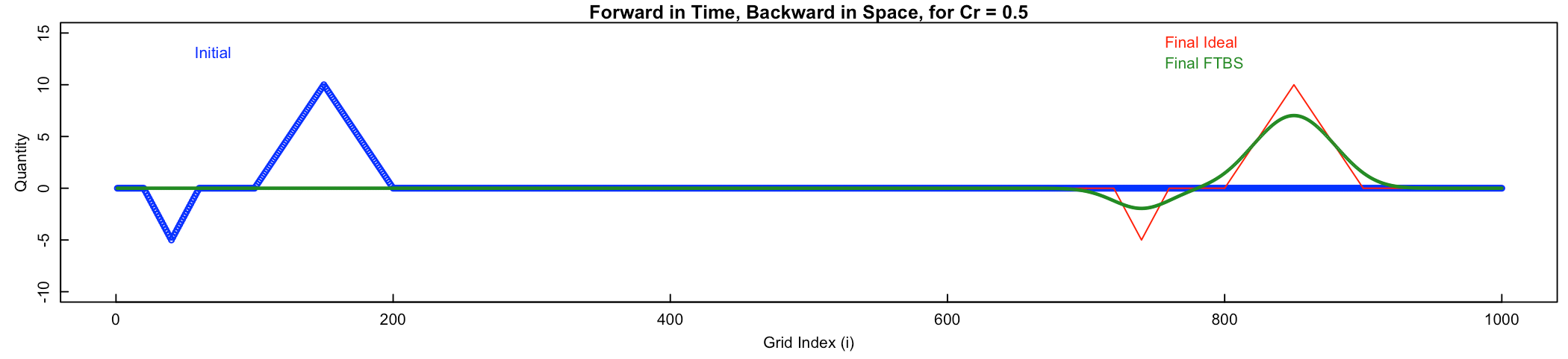
As an example, here is what the answer to Steps (2 - 4) should look like:
Under construction (this web page, and most other web pages for this course).
# In this HW 6, a 1-D pollutant puff "anomaly" is being advected in
# the x-direction by a constant wind u. The "anomaly" includes positive
# and negative concentration deviations about a mean concentration.
# [The syntax here is for the R language. Feel free to translate to
# your own favorite programming language.]
# The 3 finite-difference schemes you will compare are
# (a) FTBS - Forward in time, Backward in space;
# (b) RK3 - Runga-Kutte 3rd order, and
# (c) PPM - Piecewise Parabolic Method
# where PPM is the scheme used to advect pollutants in the CMAQ model. (see the assigned readings before class)
# Create the grid and initial conditions
imax = 1000 # number of grid points in x-direction
delx = 100. # horizontal grid spacing (m)
delt = 10. # time increment (s)
u =
5.
# horizontal wind speed (m/s)
# 1) Calculate and display the Courant number. You can display it inside
# the graph that you produce for question (3) if you would like.
# 2) (a) Create initial concentration anomaly distribution in the x-direction
# as shown as the blue line in the figure below. I did it in R using these functions:
conc <- rep(0.0, imax) # initial concentration of background is zero
cmax
=
10.0
# max initial concentration
conc[100:150] <- seq(0., cmax, len = 51) # insert left side of the upward triangle
conc[150:200] <- seq(cmax, 0., len = 51) # insert right side of upward triangle
conc[20:40] <- seq(0., -0.5*cmax, len = 21) # insert left side of downward triangle
conc[40:60] <- seq(-0.5*cmax, 0., len = 21) # insert right side of downward triangle
# (b) Plot (using blue colour) the initial concentration distribution on a graph.
# [See a sample of this output below.]
# 3) Also, on the same plot, show (in red) the ideal exact final solution,
# after the puff anomaly has been advected downwind, as given by
cideal <- rep(0.0, imax) # final concentration of ideal background is zero, except as given below:
cideal[800:850] <- seq(0., cmax, len = 51) # insert left side of positive triangle
cideal[850:900] <- seq(cmax, 0., len = 51) # insert right side of positive triangle
cideal[720:740] <- seq(0., -0.5*cmax, len = 21) # insert left side of negative triangle
cideal[740:760] <- seq(-0.5*cmax, 0., len = 21) # insert right side of negative triangle
# [See a sample of this output in the figure below.]
# 4) Given the initial puff concentration,
#
Advect the concentration puff anomaly for the following number of time steps
nsteps = (imax - 300) / (u * delt / delx)
# and plot (in green) the resulting concentration on the same graph, using ...
# "forward in time, backward in space" (FTBS) .
# [See a sample of this output below.]
# 5) Repeat steps (2-4) to re-initialize, but plotting (in green) on a new graph, and using
# RK3 for the advection. Start from the same initial condition, and use same number of time steps.
# 6) Repeat steps (2-4) to re-initialize, but plotting (in green) on a new graph, and using
# PPM for the advection. Start from the same initial condition, and use same number of time steps.
# Attached is a code fragment that shows the PPM algorithm (in R as text or as pdf) for
# our simplified homework problem. You can use or modify it to do this PPM exercise.
# It assumes you are using the variable and array names exactly as written above.
# 7) Discuss and compare the results of these three advection schemes.
As an example, here is what the answer to Steps (2 - 4) should look like: