DCIP2D:
Inversion of 2D DC Resistivity Data

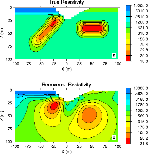
Previous Page (General Methodology for inverting DC and IP data) | Next Page (Inversion of IP Data)

The inversion of the apparent resistivity data shown in Fig 3b is carried out using the program DCINV2D. In performing this inversion we keep the same mesh for the inverse problem as for the forward problem. This means that we will find conductivities for the 1296 cells so that the 124 observations are adequately fit. In the synthetic modelling we know the standard deviation of the data errors and therefore an appropriate target value for the misfit is _d^*=124.

Our model objective function is of the form indicated in equation (9). For this particular inversion we have set w_s ,w_x ,w_z equal to unity and have chosen _s=.001, _x=1.0, _z=1.0 and m₀=1 mS/m.

The inversion method requires linearizing the data equations and iterating. The details of the inversion can be found in Oldenburg, McGillivray and Ellis (1993). At each iteration a system of equations is solved using generalized subspace techniques. The inversion begins with a halfspace of conductivity 1 mS/m and at every iteration we ask for a 50% decrease in the misfit objective function until the target misfit _d = N is achieved. Once the target misfit has been obtained, the iterations continue in an attempt to reduce the model objective function and hence reduce unnecessary structure while keeping the misfit at the desired target value. For the example presented here the desired misfit _d =124 is achieved by iteration 12 but a few more iterations are carried out until no further decrease in the model objective function is obtained. The model obtained at iteration 20 is shown in Fig 5b. It compares favorably with the true input model in Fig 5a. The surface variation is well defined and so are the conductive anomalies at depth. The conductivities toward the bottom of the model approach that of the halfspace reference model. This is the expected result. If the data are insensitive to certain regions of the model domain then the inversion will make those regions have conductivities close to the reference model as this will be most effective in reducing the value of the model objective function. To quantify the benefits of the inversion, the reader should compare the constructed model in Fig 5b with the apparent resistivity pseudo-section in Fig 3b.

Appendix: If there is a need to incorporate a known dip into the inversion, see Li, Y., and Oldenburg, D.W. (2000). There are instructions for incorporating dip with DCIP2D in a short appendix (PDF) to the manual