|
Previous Page (Forward Modelling) | Next Page (Inversion of DC Resistivity Data)
The computing programs outlined in this manual solve two inverse
problems. In the first we invert the DC potentials  (or
equivalently the data in Fig 3b) to recover the electrical conductivity (or
equivalently the data in Fig 3b) to recover the electrical conductivity
 (x,z). This is a nonlinear inverse problem that requires
linearization of the data equations and subsequent iteration. Next we
invert the IP data in Fig 4b to recover the chargeability (x,z). This is a nonlinear inverse problem that requires
linearization of the data equations and subsequent iteration. Next we
invert the IP data in Fig 4b to recover the chargeability  (x,z).
Because chargeabilities are usually small quantities ( 0.3) it is
possible to linearize equation (6) and derive a linear system of
equations to be solved. Irrespective of which data set is being inverted
however, we basically use the same methodology to carry out the
inversions. (x,z).
Because chargeabilities are usually small quantities ( 0.3) it is
possible to linearize equation (6) and derive a linear system of
equations to be solved. Irrespective of which data set is being inverted
however, we basically use the same methodology to carry out the
inversions.
To outline our methodology it is convenient to introduce a single
notation for the "data" and for the "model". We let
d = (d1,d2,...,dN) denote the data.
So di could be the ith potential in a dc resistivity data set or the
ith apparent chargeability in an IP survey. Let the physical property
of interest be denoted by the symbol m. The quantity mi can denote the
conductivity or chargeability for the ith cell. For the inversion we
choose mi = ln i when inverting for conductivities and
mi = i when reconstructing the chargeability section.
The goal of the inversion is to recover a model vector
m = (m1,m2,...,mM) that acceptably
reproduces the N observations
dobs = (d1obs,d2obs,...,dNobs) . Importantly, the data are noise
contaminated so we don't want to fit them precisely. To do so would
ensure that we do not have the correct earth model. Some features
observed in the constructed model would assuredly be artifacts of the
noise. Alternatively, if we fit the data too poorly then information
about the conductivity that is coded in the data will not have been
recovered. Our objective therefore is neither to underfit nor overfit
the data. Rather, we want to find a model which reproduces the data only
to within an amount that is justified by the estimated uncertainty in
the data. To accomplish this we introduce a global misfit criterion
 (7) (7)
where Wd is a
datum weighting matrix. In this work we shall assume that the noise
contaminating the jth observation is an uncorrelated
Gaussian random variable having zero mean and standard
deviation  j . As such, an
appropriate form for the N×N matrix is j . As such, an
appropriate form for the N×N matrix is  . With this choice, . With this choice,  d is the
random variable distributed as chi-squared with N degrees of freedom. Its
expected value is approximately equal to N and
accordingly, d*, the target misfit for the inversion, should be
about this value. d is the
random variable distributed as chi-squared with N degrees of freedom. Its
expected value is approximately equal to N and
accordingly, d*, the target misfit for the inversion, should be
about this value.
Earth conductivity distributions are complex. To allow maximum
flexibility to produce a model of arbitrary shape it is important that
M, the number of cells representing the model, is large. In our
inversions M will almost always be greater than N, the number of data.
The inverse problem therefore reduces to finding a set of M parameters
using only N data constraints under the condition that M,N. Clearly the
solution is nonunique and this nonuniqueness represents the principle
obstacle for obtaining unambiguous information about earth structure
from the observations.
Any inversion algorithm (if it works) will produce a model which
reproduces the data. But there are infinitely many models possible. So
which one does the algorithm produce? It is not good practise to let the
program make a random selection. Rather, a responsible approach is to
direct the inversion algorithm to produce a model that is geologically
reasonable and is constrained by additional information if that
information is available. This can be implemented by formulating a
"model objective function" which, when minimized, produces a model with
desirable characteristics. The critical aspect of the inversion is
therefore to form the model objective function which we characterize by
m . To do this, the inversionist must ask the question "what type of
model is desired?". Should the model be smooth, should it be blocky? Is
there a reference or background model that the constructed model should
emulate? If there is a reference model, is it better known in some
places than others so that the constructed model should be close to the
reference model in certain locations but can depart from our
preconceived ideas in other areas? Whatever the answer to these
questions, a guiding philosophy should always be to find a model which
(in some sense) is "as simple as possible". The nonuniqueness inherent
in the inversion generally means that we can generate models which are
arbitrarily complicated. We cannot however, make models that are
arbitrarily simple. For example a halfspace will generally not reproduce
data acquired from a geophysical survey.
In the inversion algorithms in DCIP2D our choice for the objective
function m is guided by a desire to find a model which has minimum
structure in the vertical and horizontal directions and at the same time
is close to a base model m0 . To accomplish this we minimize a
discretized approximation to
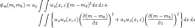 (8) (8)
In equation (8) the functions ws ,wx ,wz are specified by the user and the
constant  s controls the importance of closeness of the
constructed model to the base model m0 and x , z control
the roughness of the model in the two directions. Varying the ratio
x / z allows the construction of models that are smoother,
thus more elongated, in either x- or z-direction. The discrete form of
equation (8) is s controls the importance of closeness of the
constructed model to the base model m0 and x , z control
the roughness of the model in the two directions. Varying the ratio
x / z allows the construction of models that are smoother,
thus more elongated, in either x- or z-direction. The discrete form of
equation (8) is
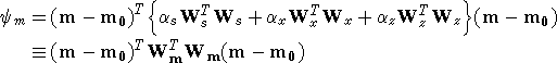 (9) (9)
If ws ,wx ,wz are set equal to unity then
Ws is a diagonal matrix with elements  where where  x is the length
of the cell
and z is its thickness, Wx has
elements x is the length
of the cell
and z is its thickness, Wx has
elements  where dx is the distance between the
centers of horizontally adjacent cells, and Wx has
elements where dx is the distance between the
centers of horizontally adjacent cells, and Wx has
elements  where dz is the distance between the
centers of vertically adjacent cells. where dz is the distance between the
centers of vertically adjacent cells.
The inverse problem is now properly formulated as an optimization
problem:
 (10) (10)
In equation (10) m0 is a base model and Wm is a general weighting matrix
which is designed so that a model with specific characteristics is
produced. The minimization of m yields a model that is close to m0 with the
metric defined by Wm and so the characteristics of the recovered model are
directly controlled by these two quantities. If the data errors are
Gaussian and their standard deviations have been adequately estimated
then Wd can be set to and the target misfit should be d* = N.
Previous Page (Forward Modelling) | Next Page (Inversion of DC Resistivity Data)
|
