After an explanation of isobaric vs. constant-height surface, scroll down to access detailed explanations of the various weather maps provided with this course via the "Forecast Tools" link in the webpage header.
The atmosphere is 5-dimensional: x, y, z, t, var. These symbols are: x = distance positive toward the east, y is distance positive toward the north, z is distance positive upward, t is time, and var indicates multiple variables such as temperature, humidity, wind, etc. It is hard to show all 5 dimensions on a 2-D computer screen, so instead we often show 2-D maps of horizontal weather (x, y), sometimes with multiple variables (var), and animated in time (t), thus allowing us to see 4 of the 5 dimensions.
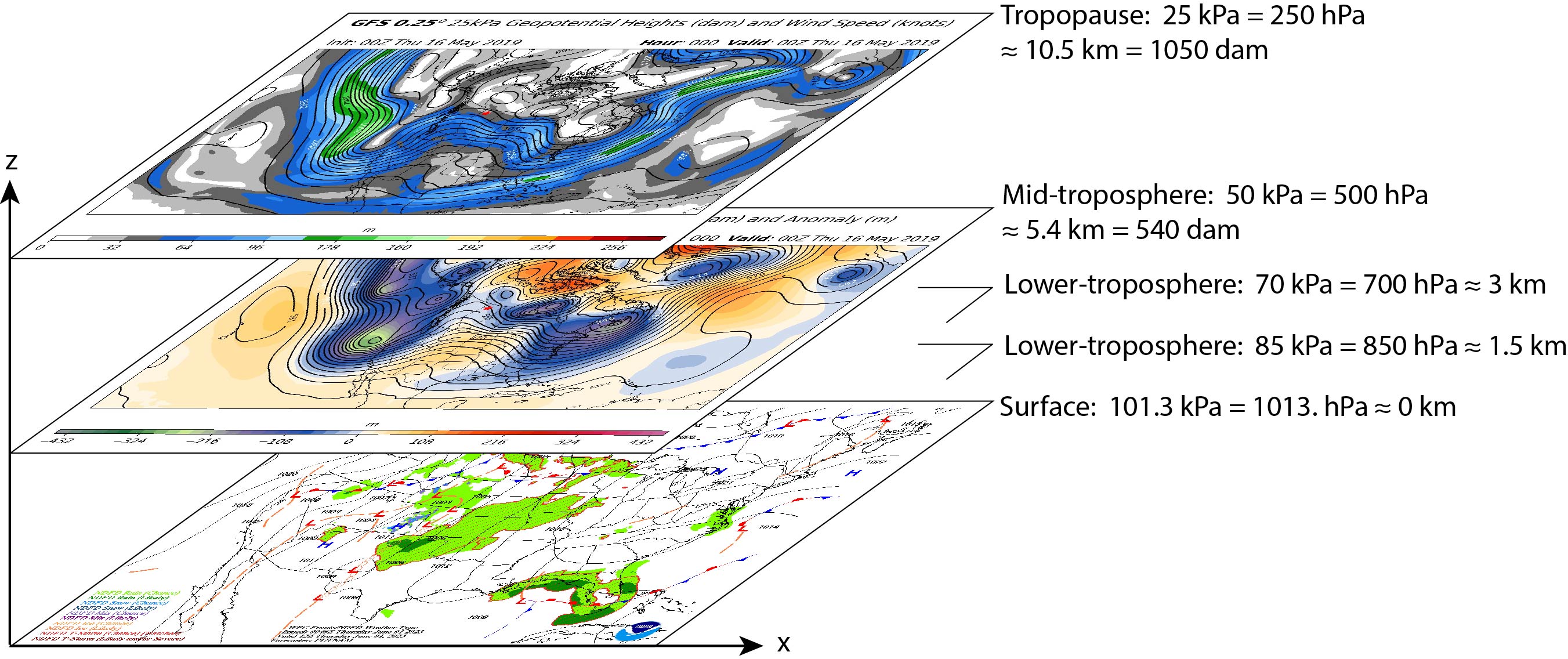
For the 5th dimension, height (z), we look at separate maps or animations for key heights. Recall that atmospheric pressure decreases monotonically with height (Practical Meteorology [PrMet], Chapter 1, section 1.4.3), allowing us to use pressure as a surrogate for height (PrMet, Ch.1, Fig. 1.4). Higher heights correspond to lower pressures. Although Fig. 1 below shows multiple maps stacked in the vertical, in reality you must look at separate maps for each height and mentally form a 3-D picture in your mind.
| Aside: Isobaric Surfaces | Aside: Init. time, Valid Time, & Forecast Skill |
|---|---|
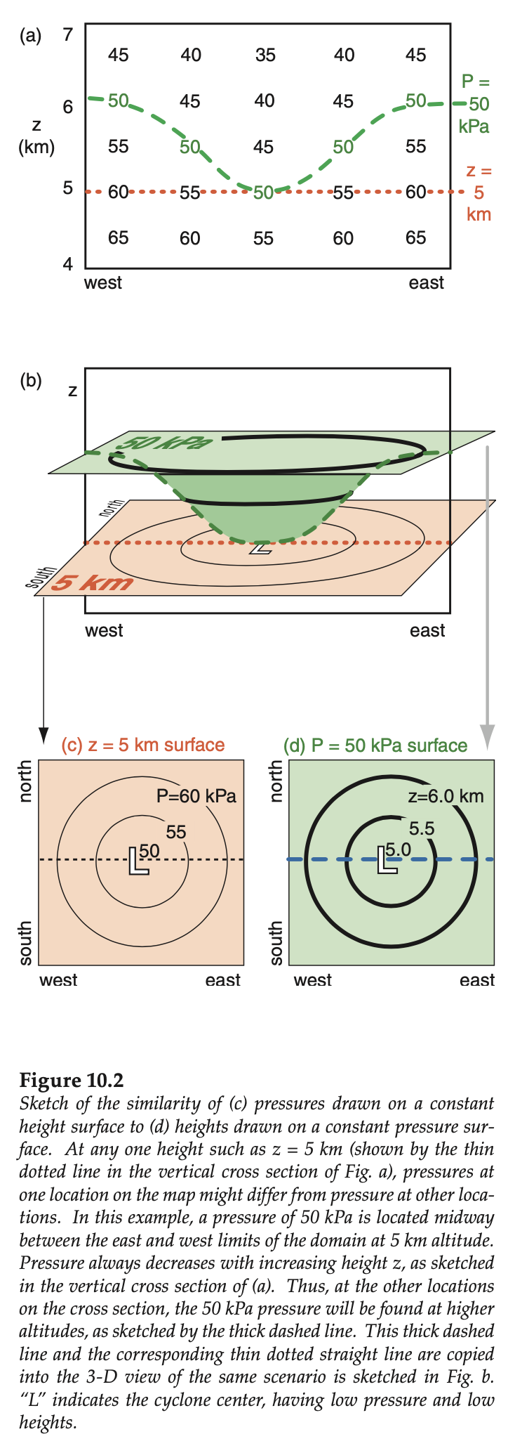
Recall that low pressures on a constant height surface correspond to low heights on an isobaric surface. The sketch below, from PrMet, Ch.10, shows this relationship.
|
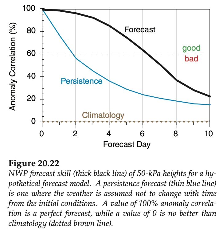
Recall that forecast skill decreases with increasing forecast horizon. Namely, the further into the future you forecast, the less skill you have. This is illustrated in Fig. 20.22 from PrMet, Ch.20.
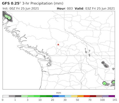
Also recall that numerical weather prediction (NWP) is an "initial value problem." Namely, we need to start with some known initial condition of the atmosphere (i.e., the "analysis", based partly on the actual observed weather). Each forecast that we make for future weather has some valid time. For example, if we initialize the model with an analysis that was valid at 00 UTC (= 00 Z) on day 1, and we forecast 36 hours into the future, then the valid time is 12 UTC on day 2. Thus, each weather map is identified with an Initialization Time (Init.), the Valid Time (Valid)of the current map, and the number of hours (Hour) between the initialization and the forecast valid time. A greater number of hours generally implies less skill. If the forecast is for Hour = 000, then you are looking at the initial analysis. Via the internet, you have access to forecasts from many different NWP models, and many different horizontal grid resolutions. For example, if a coarse-resolution (0.25° latitude ≈ 25 km) weather forecast from the Global Forecast System (GFS) model is used, then the weather map is labeled as "GFS 0.25° ". Also, do NOT use the first 3 h or so of the NWP forecast, because this is the initial "spin up" phase of the model, where the clouds and precipitation are still being created. |
| Map Name | Example |
|---|---|
| 25 kPa Geopotential Heights (dam) and Wind Speed (knots) | 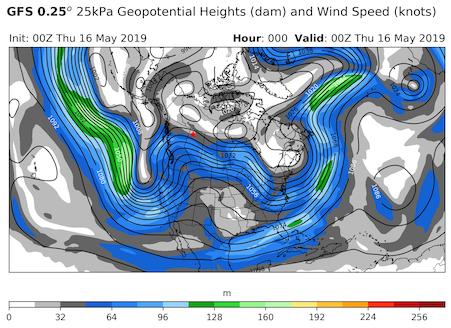 |
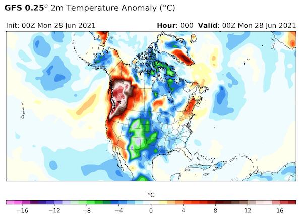
| 50 kPa Geopotential Heights (dam) and Anomaly (m) | 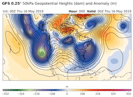 |
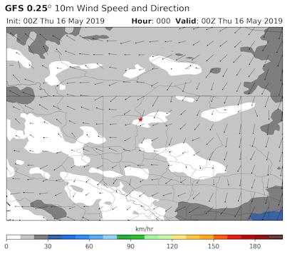
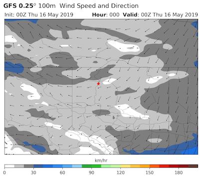
| 85 kPa Wind Speed and Direction | 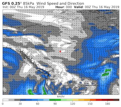 |
| Map Name | Example |
|---|---|
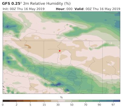
| 70 kPa Relative Humidity (%) | 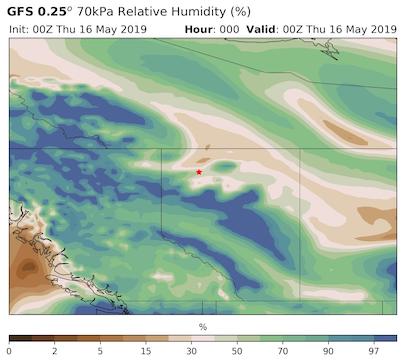 |
| Map Name | Example |
|---|---|
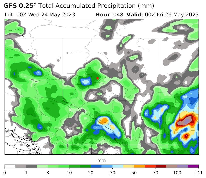
| 3-hr Precip (mm), MSLP (hPa), 100-50 kPa Thickness (dam) | 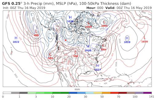 |
| Map Name | Example |
|---|---|
| Vertical Cross Sections | 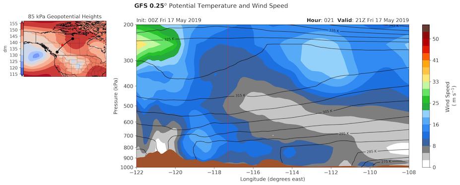 |
| Upper-level Divergence | 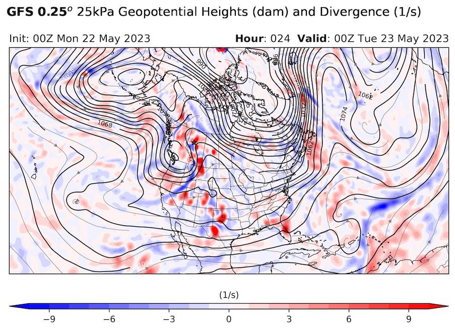 |
| xxx | |