EOSC350 Lab 1, 2011

Instructor: Doug Oldenburg, doug@eos.ubc.ca , TAs: Dikun Yang, Sarah Devriese, Mike McMillan

Purpose:

Gain familiarity with the general 7-step framework for applying geophysics. This exercise is an introduction to the various steps involved in supplying and/or using geophysical information.

Materials:

• A short online reading in GPG, Ch2.b.1.
• Displays in the Pacific Museum of the Earth (PME), in the EOS-Main building lobby.
• A simple plotting program, and an airborne magnetic survey data set, both of which you will download at step 5.

Instructions:

• Answer questions labelled with 'Qx' as briefly as possible (no essays!). Please use a word processor because you will need to paste an image into it.
• Note that sections 2, 3, & 4 involve finding stuff in the PME (Pacific Museum of the Earth).
• Due date: First lecture following your lab section (or end of lab if you can). Please hand in paper copies of your work - don't forget your name.

Questions:

1. Familiarize yourself with the 7 step framework by reading the single page at GPG, Ch2.b.1.
   1. Q1. Which one of the seven steps is considered the key link between geologic requirements and geophysical information?
   2. Q2. Why did you choose this as a key step?
        
2. Setup: We will now work on aspects of each of the 7 steps, starting with "setup" - i.e. clarifying the geoscience task and it's context.
   You will need to go down to the PME (Pacific Museum of the Earth).
   NOTE: DO NOT SPEND MORE THAN 15-20 MINUTES IN THE MUSEUM.
   1. In the PME, find the one geophysical data set that is NOT related to either the Lithoprobe project, or earthquakes.
   2. Q3. What is the geoscience task that prompted acquisition of this data set?
   3. Q4. Give one example of prior knowledge that a professional would be expected to know about, prior to doing geophysical work. No details - just an example of some type of information about this task that might be known before doing geophysical work.
        
3. Properties; Consider the geoscience task in the display you have found in the PME:
   1. Q5. What is the primary physical property that allows the survey data shown to distinguish the target from the host rocks?
   2. Q6. What is the geological structure that they are trying to locate by performing this geophysical work?
   3. In the PME's rock type displays, find one other rock that is most likely to have a high magnetic susceptibility.
      1. Q7a. What is the name of this rock?
      2. Q7b. What minerals are in the rock?
   4. Q8. Imagine that a geophysical survey is planned to map the distribution of that rock type. For this to be possible, what is one necessary characteristic of the rocks surrounding the “target”?
        
4. Surveys: Return to the geophysical data in the PME that you were referring to earlier.
   1. Q9. Which of the two data set shown is real and which is a simulation?
   2. Q10. Describe what pattern in the simulated data is characteristic of the target.

Up to this stage we have been considering the initial steps that are necessary prior to collecting geophysical data, or before data are provided by a contractor. The rest of the work involves considering the measurements and data processing, the interpretation of those data, and the impact of the geophysical data on the geoscience problem.

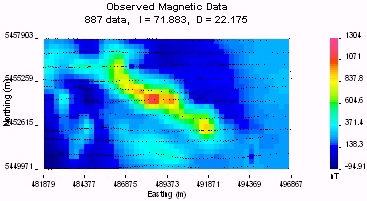
5. Data: We will make use of an airborne magnetic survey data set collected near the UBC Geology Field Camp, in the Okanagan Valley of BC.
1. Ideally you should have read the four GPG Ch2.e. pages about plotting, but if you haven't yet, plan on doing that later.
2. We want to plot survey data as a colour contour map. Click here to save a simple plotting program "gm-data-viewer" to your computer. (No further "installation" is needed).
3. To obtain the data set, RIGHT-click here (use the RIGHT mouse button) and save the file to the same place as the program.
4. Plot this data by (a) running the program then (b) opening (File=>Open) the file called "framewrk-anomaly.dat", which you should have put in the same place as the program.
5. What are we looking at?
   1. Q11. Five points to recognize are: (a) Roughly what is the area of the map? (b) How many data points are there (Hint - you don't have to count them!)? (c) How many survey lines with dots showing measurement locations are there? (d) Roughly how far apart are the survey lines (which are in fact flight paths)? (e) What is the range of measurement values (units are nanoTeslas - we'll learn what it all means later)?
6. Change the colour scale using the View=>Colour map option.
   1. Q12a. Which colour scales tend to obscure information contained in the data?
   2. Q12b. Which one scale seems to reveal the most detail across the whole range of data values?
   3. Q12c. We would like to emphasize details for the anomaly centred in the middle of the second row of data points (tiny dots) from the bottom. Change the colour scale using the Options => Max / Min ... menu, and tell us what you decided to use for Maximum and Minimum values. Why did you choose these values?
        
6. Processing: We will not actually do any data processing today. However, examples of some processing options are shown here on a separate page. Please look at that page and answer the following questions:
   1. Q13. Which processing method do you think would be most helpful in finding the geological contact between the magnetic rocks in our example and their surroundings?
        
7. Interpretation (still working with the data in the viewing program). We will compare magnetics to elevation and geology, and estimate a depth to the susceptible zone by analysing a line profile extracted through our data.
   1. Return your plot to it's "default" plotting parameters. Then, add the elevation to the plot using the View=>Elevation menu option.
   • Q14. Does there appear to be any correlation between elevation and magnetic data?
   2. Compare your plot to the corresponding region on the larger data set given on this page.
   • Q15. Which geologic unit (from the geology map's key) is most likely to be causing the main diagonal anomaly in your plot? (Hint, use grid lines to help compare the geophysics and geology maps.)
   3. Back to the data plot you have made: it should be in it's "default" mode, like the image to the right. Draw a straight line that crosses perpendicuar to the diagonal anomaly across it's strongest point. Do this by clicking inside the data plot at the start of your line and dragging to the end of the line. A line profile of the data will appear under the map. You can redo the line anytime by re-drawing it.
   • Q16. What are the maximum and minimum measured values along the line you just defined?
   • Now click carefully on the line profile graph (not the map) at half the maximum anomaly value. The width of the anomaly at this value will be given below the profile's x-axis.
   • Q17. Paste a copy of this plot (map and line profile) by (a) clicking the left-most toolbar button (or select Edit=>Copy), then (b) switching to your answer document and "pasting" the image into your document at the location you want.
   • If the anomaly was caused by a simple horizontal cylinder (a not-too terrible approximation in this case), the vertical distance between measurement location and the centre of this cylinder can be estimated using D=0.75x, where x is the anomaly's width at half it's amplitude.
   • Q18. If the survey had been carried out with sensors at 300m above the surface, what would the depth (below ground surface) to the simplified cylinder model be?
   There is plenty more we could do with these data, but we are running out of time for this exercise.
     
8. Synthesis: This is when geophysical work is correlated with everything else known about the problem. Click to open the multiple maps page (in a new window) and answer the following multiple choice questions.
    
   Q20A to Q20H: In your answer document, simply enter a list of question numbers with your choice for each.
   

   Satellite images provide many types of insight. For example, does it appear as if our area of interest is mainly forested or clear? forested clear What other land-use information might affect decisions about exploration or geologic activity in any given area? Locations of Old Growth Management Areas Locations of regional parks proximity to municipalities and suburbs Ranching and other agricultural activity all of these, and perhaps others What is our area’s “metallic mineral potential” - ie, it’s mineral ranking? Highest Next to highest Moderate Lowest Are there any known controls on geologic structure through our area (ie faults)? none extensional faults normal faults thrust faults other types of fault

   What is the geochemical evidence for base metals in streams of our area? strong moderate weak non existant What is the dominant rock type in our area? intrusives metamorphics sediments volcanics Are there any measured ages of rocks in our area? yes no With the understanding about magnetic data you have gained throughout this exercise, how useful do you think the public domain image of aeromagnetics is? Suggests general trends at the regional scale. Gives indications of structures at the scale ofa few kilometers. Yields high resoution details about features at the scale of 100's of metres. Is no use at any scale.



9. Carry out a visual comparision between the regional aeromagnetics map and the maps showing the varries types of rock units (volcanics, metamorphics, sedimentary, and intrusive).
   • Q21a. Which rock units are associated with highs in the magnetic data?
   • Q21b. Which rock units are associated with lows in the magnetic data