| |
Related documentation:
| DCIP2D user interface | data viewer | model maker | model viewer | tutorial |
The program called dcip2d-dataviewer.exe displays observed data as a pseudosection, and optionally a second pseudosection representing either predicted data, the data error map, or the difference between observed and predicted data normalized by standard deviation. The image can be adjusted or copied and data errors can be specified globally or individually.
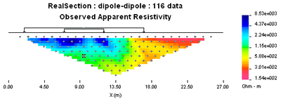
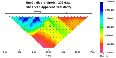
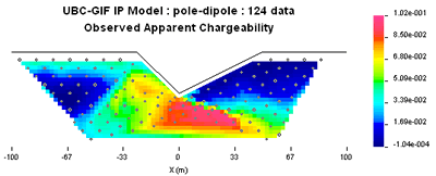
Examples of data displayed as pseudosections are shown to the right. Array types this program can display are as follows.
- dipole-dipole
- pole-dipole
- dipole-pole
- pole-pole
- RealSection or Wenner: **New, Dec 2005 ('experimental') - to view Wenner or Realsection data, enter RealSection for the TITLE and dipole-dipole for TYPE.
Starting this program
This tool is run in either of three ways:
1) Press the View data / Errors button in the Observations section of the DCINV2D control window to inspect raw data.
2) Press the Pre button on the DCINV2D control windows's tool bar, when inversion is either under way, or is finished. Raw data, predicted data, errors and misfit can all be examined, adjusted and copied.
3) The program can also be run directly. Use the File menu, Open ... option to view raw data files. If "dcip2d-data-viewer.exe" is run from the command line with no parameters (or by double clicking it's icon) it will open directly with a blank window. However, a data set can be loaded directly using the following command line parameters:
dcip2d-data-viewer datafile /dc /ip /topo=topofile /pre
/dc - DC data.
/ip - IP data.
/topo="filename" - read topography from topofile - INCLUDE QUOTES!
/pre - read the predicted data file ("dcinv2d.pre" or "ipinv2d.pre")
NB: Currently the only way to display topography is to run the program from the command line. Do not forget to add the double quotes for topography's filename.
Menu functions
Most menu options are duplicated with buttons on the tool bar. Exceptions include:
- The Options menu, Min/max ... function is used to adjust the range of values depicted by the colour scale. It is useful if need to compare several figures.
- The Options menu, IP units ... permits you to change the label (only) on the colour scale.
- The Edit menu, Add Errors ... option is described below under Individual datum errors.
- The View menu Flip Colours option changes the colour bar from red through blue to blue through red.
Tool bar functions
- The open button asks you to specify an observations data file and whether the data are DC or IP. New March 2007: You can also optionally include a predicted data file and a topography file in DCIP2D top.dat file format (specified in the user manual).
- The save button saves the current data file. It is used after adjusting errors. It does NOT save the image in any way.
- The copy button places an image of the window into the Windows95 clip-board. It can then be "pasted" into a document or paint program for saving or manipulating.
- The Log10, / , and Colour / BW buttons are toggles that affect the colour bar and the image titles.
- The two zoom buttons help you adjust figures to smaller sizes when copying, or larger for more convenient viewing on the screen.
- The Error, pre, and diff buttons select what is displayed below the raw data pseudosection. They are only available after an inversion has begun because they use information generated by the inversion program.
Standard deviations (errors) for data
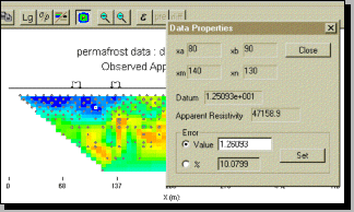 Details of individual data points are obtained by pointing carefully to a dot on the observed data pseudo-section and clicking. The source and receiver electrode locations are displayed on the pseudosection, and a dialogue box appears showing position, value, and details about error statistics for the datum. This permits adjustment of standard deviations specified for individual data points. Details of individual data points are obtained by pointing carefully to a dot on the observed data pseudo-section and clicking. The source and receiver electrode locations are displayed on the pseudosection, and a dialogue box appears showing position, value, and details about error statistics for the datum. This permits adjustment of standard deviations specified for individual data points.
Standard deviations for all data can be adjusted globally using the Edit menu, Add Errors ... option. Recall that the error component of a datum, e, assigned to any datum, x, is generally described as e = ax + b where a is a percentage (10% is entered as 10) and b is an offset in the units of data (volts or chargeability) which makes smaller data values have larger assigned errors. Values entered in the error adjustment dialogue will be assigned to all of the currently displayed data. For DC resistivity, entering a value of 0.01 in the "+minimum" box means that 10 millivolts is to be the offset component of assigned standard deviations. Values entered in the error adjustment dialogue will be assigned using e = ax + b to all of the currently displayed data.
NOTE: After adjusting any error values, you must press the Save button before using the data in an inversion.
Standard format for resistivity or IP data:
A record for each datum is stored on one line. Each record consists of six columns specifying the locations of the current electrodes (XA,XB) and potential electrodes (XM,XN), data (units of voltage) and standard deviation (optional). The data records (rows) can be arranged in any order. The file structure for the standard format obs.dat is as follows:
TITLE
TYPE
XA1 XB1 XM1 XN1 VAL1 ERR1
XA2 XB2 XM2 XN2 VAL2 ERR2
XA3 XB3 XM3 XN3 VAL3 ERR3
:
- TITLE
- this line is not usually used in the programs. It is a file header describing the data. It must be on the first line of the file and cannot be preceded by blanklines. (New, Dec 2005 ('experimental') - to view Wenner or Realsection data, enter RealSection for the TITLE and dipole-dipole for TYPE.)
- TYPE
- type of electrode configuration. This should be one of the following four values:
- pole-pole,
- pole-dipole,
- dipole-pole,
- dipole-dipole,
- New, Dec 2005 ('experimental') - to view Wenner or Realsection data, enter RealSection for the TITLE and dipole-dipole for TYPE.
where the first word denotes the configuration of the corrent electrodes and the second word denote the potential electrodes. For example, pole-dipole means current is input by a pole and potential is measured by a dipole. For Wenner, Schlumberger, gradient or irregular arrays, specify dipole-dipole and ensure that all current and potential electrode positions are specified explicitly. See the GUI documentation for more details.
- XAi, XBi
- X positions (in metres) of the current electrodes used to measure the datum VALi. When current is input by a dipole, XB will be taken as the position of the negative current electrode. When current is input by a pole, XB is not used, but the input field must remain.
-
XMi, XNi
- X positions (in metres) of the potential electrodes used to measure the datum VALi. When potential is measured by a dipole, XN will be taken as the position of the negative potential electrode. When potential is measured by a pole, XN is not used, but the input field must remain.
-
VALi
- value of observed datum. The potential measurements must be measured value in Volts for potential, or a dimensionless real number (not percentage) for apparent chargeability. (The potential value is always normalized to unit current amplitude.) There are four types of IP data generally in use; two gathered in the time domain and two gathered in the frequency domain. For small chargeabilities, as is nearly always the case for earth materials, all data types can be used as input for inversion, and resulting models will have chargeabilities in the same units.
-
ERRi
- standard deviation of the datum VALi. This is an absolute value and should not be specified as a percentage. This value should always be positive. If the first datum does not have an error field (or the error field is commented out by placing a "!" before it), the default errors for the entire data set will be calculated from the data.
|
|