| |
Related documentation:
| DCIP2D user interface | data viewer | model maker | model viewer | tutorial |
This page provides a quick tutorial describing how to install and run DCIP2D using the graphical user interface (GUI).The GUI operates only on computers running MS Windows operating system (versions 95 - through XP). The meaning of all the inversion parameters in not explained in this file. Read the main DCIP2D documentation for an explanation of the parameters.
A DC resistivity inversion must be run before any IP inversion is attempted.
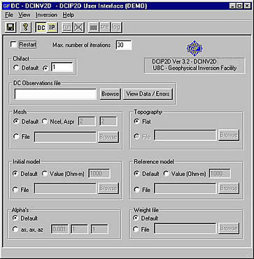
- Start up the interface to DCIP2D by executing dcip2d-gui.exe. A window will pop up reminding you of the licensing rules. Click on OK. A main window will now appear where the user should enter the inversion parameters. From now on, this window will be referred to as the "main window".
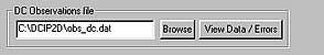
- In the "DC Observations file" field type the name of the DC data file or click on the "Browse" button to select the data file. With pre-2007 versions of the codes, there may be problems with path and file names containing space characters or that total more than 80 characters.
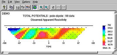
- Click on "View Data/Errors" to look at the DC pseudosection. You can close this window when done.
- Go back to the main input window. Before starting the inversion of the data you viewed in step (2), the parameters must be saved first. Click on the "Save" button
 . Save the file in the directory (ie folder) where you want to run the inversion. This is also where all of the output files will be stored. . Save the file in the directory (ie folder) where you want to run the inversion. This is also where all of the output files will be stored.
Important: It is not possible to specify output file names therefore you must use directories to keep separate inversion runs from overwriting earlier work.
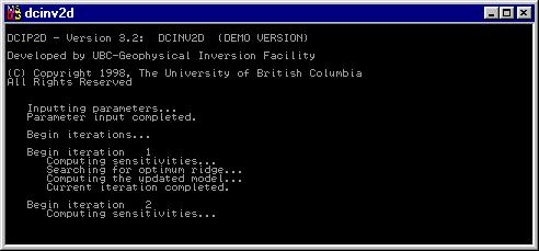
- To start the DC inversion, click the "run" button
 . A window will now appear where the progress of the inversion is displayed. . A window will now appear where the progress of the inversion is displayed.
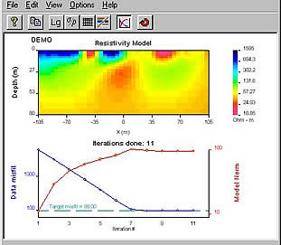
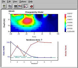
- After the first iteration is performed, you can view the model by clicking on the "model" button
 in the main window. A new window will pop up with the inverted model. in the main window. A new window will pop up with the inverted model.
In the model window you can:
- Click on the "update" button
 to update the model after each iteration. to update the model after each iteration.
- Click on the "convergence curves" button
 to view the data misfit and model norm curves. to view the data misfit and model norm curves.
- Click on the "mesh" button
 to view the mesh. to view the mesh.
When viewing the mesh, you will see that there are large padding cells on the sides of the model. To remove these cells so that you can see only the inside of the model, click on "padding cells ..." in the "Options" menu. Type the number of horizontal and vertical cells you want removed (4 or 5 are typical).
- After the DC inversion finishes, you can:
- Look at the final inverted model (see step 6).
- Look at the log file by clicking on the "log" button
 . .
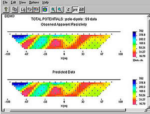
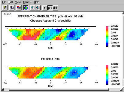
- Compare the observed and predicted data by clicking on the "pre" button
 . You might want to maximize this window to view all the information. . You might want to maximize this window to view all the information.
In this data window, you can:
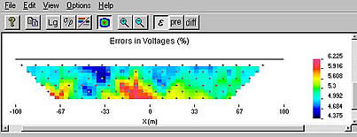
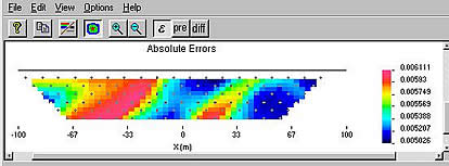
- look at the errors used in the inversion by clicking the "errors" button
 . .
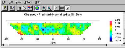
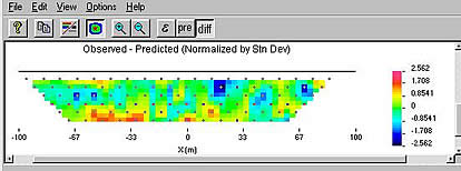
- look at the difference between observed and predicted data by clicking on the "diff" button
 . .
IP INVERSION
- Once you're satisfied with the DC inversion, you can proceed to invert IP data by clicking on the "IP" button
 on the main window. The main window will now change so that you can now invert IP data. on the main window. The main window will now change so that you can now invert IP data.
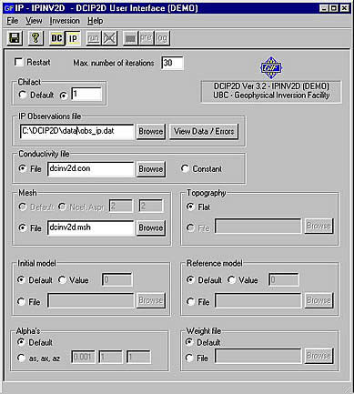
- In the "IP Observations file" field type the name of the IP data file or click on the "Browse" button to select the data file.
- IP inversion requires that a conductivity model be specified. This is usually a DC resistivity inversion result. However, a preliminary IP inversion can be run assuming a uniform conductivity by clicking the "constant" radio button.
NOTE: It is not recommended that final interpretations be carried based on IP inversion results that did not incorporate a proper conductivity model.
- The steps to invert the IP data are similar to the steps to invert the DC data. Follow steps (3) to (7) above and substitute IP for DC where appropriate. The following are the results of an IP inversion:
- You have now inverted the supplied DC and IP data with mostly default parameters. You are encouraged to redo this tutorial, but this time experiment by changing things like the reference model, errors, chifact, mesh, etc. See how these changes affect the final model.
- After redoing the inversion with a different reference model, you can view the depth of investigation by selecting this from the "Options" menu in the model viewer window.
How to change data errors:
The supplied data files do not have any errors since the last column where the errors are stored is missing. This causes the inversion programs to estimate the default errors. However, this might not always be a good choice.
To easily add errors to the data:
- Bring up the data window. Look at step (3) above.
- Click on the errors button (third from the right). If there are no errors, all of the values on the bottom plot will be zero.
- From the "Edit" menu, choose "Add Errors ...". Enter the percent and minimum. For example, if you enter the values 5 and 0.001, the error will be calculated for all data as:
error = data´0.05 + 0.001 .
- To change an error value for an individual datum, in the pseudo-section plot, click on the data whose error you want to change. A "Data Properties" window will come up were you can change the error. A good use for this is, if you have a bad data point, you can assign a large error to it.
- Once you have added the errors, you have to save the data file by choosing "Save ..." in the "File" menu. If you save the data file under a different filename than the original, make sure you update the "Observations file" field in the main window.
|
|
